12 Elements

Elements are named objects placed in three dimensions and assembled into a LINE. Shared concepts are described once; select OPALX or OPAL above for version-specific interfaces.

The OPALX view covers every element type found in the current source registry, including interfaces without maintained regression inputs. It was audited in opalx/src/OpalConfigure/Configure.cpp at source commit d1e762f15a2a. Regression coverage is stated separately from parser registration.

Type	Regression use	External data
`DRIFT`	Field-free transport	none
`CONSTANTEFIELDCAVITY`	Uniform electric field	none
`QUADRUPOLE`	Normalized quadrupole	none
`MULTIPOLE`	Normalized dipole/quadrupole arrays	none
`MULTIPOLET`	Physical multipole coefficients with fringe fields	optional time model
`SOLENOID`	Mapped solenoid field	field map
`RFCAVITY`	Standing-wave RF field	field map
`TRAVELINGWAVE`	Traveling-wave RF field	field map
`LASER`	Source registered; no maintained regression input	none
`MONITOR`	Source registered; no maintained regression input	output file
`MARKER`	Source registered; no maintained regression input	none
`PROBE`	Source registered; no maintained regression input	output file
`RBEND`, `SBEND`	Source registered; no maintained regression input	none
`VERTICALFFAMAGNET`	Source registered; no maintained regression input	none
`VARIABLE_RF_CAVITY`	Source registered; no maintained regression input	time models

The Element Physics chapter contains derivations and benchmarks where available.

12.1 Common element syntax

Every element uses

name: ELEMENTTYPE, L=length, placement, type_specific_parameters;

and accepts the following common attributes.

Parameter	Default	Current behavior
`L`	unset (\(0\,\mathrm m\) when read)	Nominal element length. Use a positive value for the element kernels documented here.
`ELEMEDGE`	unset	Places the entrance at path length \(s\) in metres. May be combined with `PSI`, but not with absolute pose attributes.
`X`, `Y`, `Z`	`0 m`	Absolute lab-frame origin. Explicitly set at least one of `X`, `Y`, `Z`, `THETA`, or `PHI` to select pose placement.
`THETA`, `PHI`, `PSI`	`0 rad`	Absolute rotations about local \(y\), \(x\), and \(z\). `PSI` is also the optional roll for `ELEMEDGE` placement.
`DX`, `DY`, `DZ`	`0 m`	Local translational misalignment applied after placement.
`DTHETA`, `DPHI`, `DPSI`	`0 rad`	Local rotational misalignment.
`APERTURE`	`ELLIPSE(1,1)` equivalent	Transverse aperture string, for example `CIRCLE(0.02)`, `ELLIPSE(0.03,0.02)`, `RECTANGLE(0.03,0.02)`, or `SQUARE(0.02)`. Dimensions are full widths in metres.
`DELETEONTRANSVERSEEXIT`	`TRUE`	Requests particle deletion when an element reports a transverse aperture exit.
`TYPE`	unset	Type-specific design selector; currently relevant to `RFCAVITY` below.
`WAKEF`, `PARTICLEMATTERINTERACTION`, `OUTFN`	unset	Parsed common compatibility attributes, but not acted on by the eight element implementations on this page.

Exactly one placement strategy is required. Supplying both ELEMEDGE and an absolute pose fails; supplying neither also fails. PSI alone does not select absolute placement.

12.2 `DRIFT`

DRIFT defines a field-free interval. It advances particles only through the normal tracker integration and provides the reference-path geometry between active elements.

D1: DRIFT, L=0.5, ELEMEDGE=0.0;

Parameter	Default	Current behavior
`L`	unset	Drift length in metres; use a positive value.
`GEOMETRY`	unset	Parsed boundary-geometry name, but not transferred by the current `DRIFT` implementation.
`NSLICES`	`1`	Map-tracking compatibility value; inactive in the current `PARALLEL` tracking path.

12.3 `CONSTANTEFIELDCAVITY`

CONSTANTEFIELDCAVITY adds a uniform Cartesian electric field over its local body interval. It is a DC element and is not processed by the RF autophaser.

Gun: CONSTANTEFIELDCAVITY,
    L=0.5, ELEMEDGE=0.0,
    EX=0.0, EY=0.0, EZ=-5.0;

Parameter	Default	Unit	Current behavior
`EX`	`0`	MV/m	Uniform local \(E_x\).
`EY`	`0`	MV/m	Uniform local \(E_y\).
`EZ`	`0`	MV/m	Uniform local \(E_z\). A negative value accelerates electrons toward local \(+z\).

The field is applied for local \(0<z\le L\) in the particle kernel. Use RFCAVITY or TRAVELINGWAVE when an oscillating mapped RF field is required.

12.4 `QUADRUPOLE`

QUADRUPOLE is a convenience wrapper around MULTIPOLE. It converts normalized strengths to physical gradients using the reference rigidity.

Q1: QUADRUPOLE, L=0.5, ELEMEDGE=0.0, K1=0.54;

Parameter	Default	Unit	Current behavior
`K1`	`0`	\(\mathrm m^{-2}\)	Normal normalized quadrupole strength.
`K1S`	`0`	\(\mathrm m^{-2}\)	Skew normalized quadrupole strength.
`DK1`	`0`	\(\mathrm m^{-2}\)	Parsed and stored normal error, but not applied by the current field kernel.
`DK1S`	`0`	\(\mathrm m^{-2}\)	Parsed and stored skew error, but not applied by the current field kernel.

Use a positive L. Although inherited help text mentions integrated zero-length strengths, the current particle kernel has no nonzero field interval when L=0.

12.5 `MULTIPOLE`

MULTIPOLE accepts arrays of normalized normal and skew strengths. Array index zero is dipole and index one is quadrupole.

M1: MULTIPOLE, L=0.5, ELEMEDGE=0.0, KN={0.0,0.54};

Parameter	Default	Current behavior
`KN`	empty	Normal normalized strengths: index 0 dipole, index 1 quadrupole.
`KS`	empty	Skew normalized strengths with the same indexing.
`DKN`	empty	Parsed and stored normal-error array, but not applied by the current field kernel. Missing entries are padded with zero.
`DKS`	empty	Parsed and stored skew-error array, but not applied by the current field kernel. Missing entries are padded with zero.

Current order limit

The parser accepts longer arrays, but the current particle and reference kernels do not agree: the bulk particle kernel applies only indices 0 and 1, while the host/reference kernel evaluates higher orders. A higher-order entry can therefore change the threaded reference orbit without applying the same field to tracked particles. Use MULTIPOLET instead.

Strengths are multiplied by the reference rigidity before tracking. As for QUADRUPOLE, use positive length; zero-length integrated operation is not effective in the current parallel kernel.

12.6 `MULTIPOLET`

MULTIPOLET defines straight or constant-radius curved magnetic multipoles using physical field coefficients and a smooth fringe model. It is distinct from the normalized MULTIPOLE interface.

MT1: MULTIPOLET,
    L=0.5, ELEMEDGE=0.0,
    TP={0.0,1.80},
    LFRINGE=0.05, RFRINGE=0.05,
    HAPERT=0.04, VAPERT=0.04;

Parameter	Default	Unit	Current behavior
`TP`	empty	\(\mathrm T\,\mathrm m^{-k}\)	Physical coefficients \(b_k\): index 0 dipole field, index 1 quadrupole gradient, and higher orders through index 5.
`LFRINGE`, `RFRINGE`	unset	m	Left and right tanh-fringe length scales. Set positive values.
`HAPERT`, `VAPERT`	unset	m	Internal horizontal and vertical aperture dimensions used by this field model.
`MAXFORDER`	`3`	terms	Longitudinal fringe expansion order. Must be in \([1,9]\); real input is converted to an integer.
`MAXXORDER`	`20`	terms	Polynomial expansion order used by the curved implementation; real input is converted to an integer.
`ROTATION`	unset	rad	Rotation about the central axis for a straight skew element. Must be zero when `ANGLE` is nonzero.
`EANGLE`	unset	rad	Entrance angle for curved geometry.
`BBLENGTH`	unset	m	Half-length used for the field calculation’s bounding region.
`ANGLE`	`0`	rad	Nonzero selects the constant-radius curved implementation; zero selects straight geometry.
`VARRADIUS`	`FALSE`	Boolean	Variable-radius selector. Variable-radius curved magnets are currently rejected.
`ENTRYOFFSET`	`0`	m	Accepted only with `VARRADIUS=TRUE`; there is no supported variable-radius curved configuration yet.
`SCALING_MODEL`	unset	name	Optional `TIMEDEPENDENCE` object multiplying the magnetic field as a function of time.

The dedicated HAPERT and VAPERT values configure this model’s internal aperture; do not substitute the common APERTURE string for them. The six-entry TP capacity is a runtime limit even though the parser accepts a longer array.

12.7 `SOLENOID`

SOLENOID loads a magnetic field map and scales it with a normalized solenoid strength. The map defines the actual longitudinal field-support interval, which may differ from nominal L.

S1: SOLENOID,
    L=0.5, ELEMEDGE=0.0,
    KS=0.12, FMAPFN="solenoid.T7";

Parameter	Default	Current behavior
`KS`	unset (\(0\) when read)	Normalized field-map scale in \(\mathrm m^{-1}\). It is converted using the reference rigidity.
`DKS`	unset (\(0\) when read)	Additive scale error for tracked particles; the reference-particle field omits this error.
`FMAPFN`	unset	Required field-map filename. Tracking cannot apply a solenoid without a loaded map.
`FAST`	`TRUE`	Passed to the field-map loader as its fast/accuracy selection.

The element does not generate an analytic hard-edge solenoid when FMAPFN is missing. Keep the field map beside the input or use an unambiguous relative path.

12.8 `RFCAVITY`

RFCAVITY applies a time-dependent standing-wave field from a supported 1D or 2D dynamic field map. The autophased example shows the complete connection to a beam and tracker.

Gun: RFCAVITY,
    L=0.2927, ELEMEDGE=0.0,
    TYPE="STANDING", VOLT=60.0,
    FREQ=1300.0, LAG=0.0,
    FMAPFN="fieldmaps/DriveGun.T7";

Parameter	Default	Unit	Current behavior
`TYPE`	unset	name	`STANDING` is the maintained regression configuration. `SINGLEGAP` is recognized internally; other common design strings fall back to standing-wave behavior.
`VOLT`, `DVOLT`	unset	MV	Nominal field-map amplitude and additive amplitude error.
`FREQ`	unset	MHz	RF frequency. A field-map value differing by more than 1% replaces it with a warning.
`LAG`, `DLAG`	unset	rad	Nominal phase and additive phase error.
`FMAPFN`	unset	path	Required dynamic field map. Current particle application supports `FM2DDynamic` and `Astra1DDynamic` maps.
`FAST`	`TRUE`	Boolean	Passed to the field-map loader.
`APVETO`	`FALSE`	Boolean	If true, excludes this cavity from automatic phase optimization.
`DESIGNENERGY`	`-1`	MeV	Positive target exit kinetic energy; the autophaser also adjusts amplitude to reach it. Negative disables the target.
`GEOMETRY`	unset	name	Parsed boundary-geometry compatibility attribute; not connected by the current update path.
`RMIN`, `RMAX`, `ANGLE`, `PDIS`, `GAPWIDTH`, `PHI0`	unset	mm or deg	Cyclotron-cavity compatibility inputs; not used by ordinary `PARALLEL` RF-field application.
`PHASE_MODEL`, `AMPLITUDE_MODEL`, `FREQUENCY_MODEL`	unset	name	Names are stored, but ordinary `RFCAVITY` tracking does not currently resolve them into time-dependence objects.

The instantaneous map scale is set by the configured amplitude and \(\cos(2\pi f t+\mathrm{LAG})\); the magnetic map component uses the corresponding sine factor. OPTION.AUTOPHASE>0 searches the reference-particle phase for maximum exit energy, using the option value as the number of refinement passes.

12.9 `TRAVELINGWAVE`

TRAVELINGWAVE applies a mapped traveling-wave RF structure. It shares the autophase controls with RFCAVITY and additionally describes the repeated-cell geometry.

TW1: TRAVELINGWAVE,
    L=2.8, ELEMEDGE=0.5,
    VOLT=15.0, FREQ=2998.0, LAG=0.0,
    FMAPFN="traveling-wave.T7",
    NUMCELLS=84, MODE=0.3333333333;

Parameter	Default	Unit	Current behavior
`VOLT`, `DVOLT`	unset	MV/m	Nominal field-map amplitude and additive error.
`FREQ`	unset	MHz	RF frequency converted internally to angular frequency.
`LAG`, `DLAG`	unset	rad	Nominal phase and additive phase error.
`FMAPFN`	unset	path	Required traveling-wave field map.
`FAST`	`TRUE`	Boolean	Passed to the field-map loader.
`APVETO`	`FALSE`	Boolean	Excludes the structure from automatic phase optimization when true.
`NUMCELLS`	unset	cells	Number of cells, converted from real input to an integer. Use a positive integer.
`MODE`	`1/3`	turns	RF phase advance between neighboring cells, expressed as a fraction of \(2\pi\).
`DESIGNENERGY`	`-1`	MeV	Positive autophaser target exit kinetic energy; negative disables the target.

Use a regression-matched map, cell count, and mode as one consistent set. As with RFCAVITY, AUTOPHASE=0 disables phase searching globally and APVETO=TRUE disables it for this element only.

12.10 `LASER`

LASER defines a passive analytic laser pulse. It is registered by the current source but is not exercised by the maintained regression suite.

L1: LASER, L=0.0, ELEMEDGE=0.0,
    WAVELENGTH=800e-9, PULSEENERGY=1.0,
    PULSELENGTH=30e-15, WAISTX=20e-6, WAISTY=20e-6,
    DIR={0,0,-1}, STOKES={1,0,0};

Parameter	Unit	Constraint
`WAVELENGTH`	m	Required and greater than zero.
`PULSEENERGY`	J	Required and greater than zero.
`PULSELENGTH`	s	Required and greater than zero.
`WAISTX`, `WAISTY`	m	Required and greater than zero.
`DIR`	none	Required nonzero three-vector; OPALX normalizes it.
`STOKES`	none	Optional three-vector with \(\xi_1^2+\xi_2^2+\xi_3^2\le1\).
`L`	m	Optional non-negative body length.

12.11 `MONITOR`

MONITOR records bunch crossings at a lattice location.

M1: MONITOR, L=0.01, ELEMEDGE=0.5, TYPE=SPATIAL, OUTFN="monitor.h5";

Parameter	Default	Current behavior
`L`	at least `0.01` m at update	Physical collection interval.
`TYPE`	non-`TEMPORAL`	`TEMPORAL` selects temporal collection; every other value selects spatial collection.
`OUTFN`	unset	Output filename passed to the monitor implementation.

12.12 `MARKER`

MARKER identifies a lattice location without adding a field. It accepts the common placement attributes. Built-in #S and #E markers denote the start and end of a line.

IP: MARKER, ELEMEDGE=1.2;

12.13 `PROBE`

PROBE records particle crossings over a rectangular span.

P1: PROBE, L=0.001, ELEMEDGE=0.8,
    XSTART=-10, XEND=10, YSTART=-10, YEND=10,
    STEP=1, OUTFN="probe.h5";

Parameter	Unit	Current behavior
`XSTART`, `XEND`	mm	Horizontal endpoints, converted to metres.
`YSTART`, `YEND`	mm	Vertical endpoints, converted to metres.
`STEP`	mm	Sampling step; default `1`.
`WIDTH`	mm	Accepted but not used by the current update path.
`OUTFN`	path	Output filename.

12.14 `RBEND` and `SBEND`

RBEND defines rectangular bend geometry whose L is the straight body length. SBEND defines sector geometry whose L is the design-orbit arc length. Both apply normal and skew components through octupole order.

B1: SBEND, L=0.5, ELEMEDGE=1.0, ANGLE=0.1,
    K1=0.0, HGAP=0.02, FINT=0.5;

Parameter	Unit	Current behavior
`ANGLE`	rad	Requested bend angle.
`K0`, `K0S`	\(\mathrm m^{-1}\)	Normal and skew dipole coefficients. If `K0` is omitted, OPALX derives the normal dipole from `ANGLE` and geometry.
`K1`, `K1S`	\(\mathrm m^{-2}\)	Normal and skew quadrupole coefficients.
`K2`, `K2S`	\(\mathrm m^{-3}\)	Normal and skew sextupole coefficients.
`K3`, `K3S`	\(\mathrm m^{-4}\)	Normal and skew octupole coefficients.
`HGAP`	m	Half gap; OPALX stores twice this value as the full gap.
`FINT`	none	Fringe integral; default `0.5`.
`HAPERT`	m	Positive values install a rectangular transverse aperture.
`DESIGNENERGY`	eV	Optional design energy forwarded to the bend.
`E1`, `E2`	rad	Parsed but explicitly rejected by the current native bend port.
`GAP`, `GREATERTHANPI`	-	Rejected compatibility attributes. Use `HGAP`; bends beyond the old compatibility path are unsupported.
`WAKEF`, `PARTICLEMATTERINTERACTION`	name	Rejected by the current native bend port.

The classes are registered but currently lack maintained regression inputs. Treat pole-face, fringe, aperture, and sign conventions as experimental until validated for the intended lattice.

12.15 `VERTICALFFAMAGNET`

VERTICALFFAMAGNET defines a vertical fixed-field alternating-gradient magnet with a tanh longitudinal fringe.

Parameter	Unit	Meaning
`B0`	T	Nominal dipole field at zero height.
`FIELD_INDEX`	\(\mathrm m^{-1}\)	Exponential vertical field index.
`WIDTH`	m	Full horizontal aperture width.
`MAX_HORIZONTAL_POWER`	integer	Highest horizontal expansion power.
`END_LENGTH`	m	Tanh fringe length.
`CENTRE_LENGTH`	m	Flat-top length.
`BB_LENGTH`	m	Bounding-box length.
`HEIGHT_POS_EXTENT`, `HEIGHT_NEG_EXTENT`	m	Positive and negative vertical aperture extents.

This registered element has no maintained OPALX regression input; validate its placement and field before production use.

12.16 `VARIABLE_RF_CAVITY`

VARIABLE_RF_CAVITY applies a hard-edge electric field whose phase, amplitude, and frequency are supplied by named time-dependence definitions.

VC1: VARIABLE_RF_CAVITY, L=0.2, ELEMEDGE=0.0,
     PHASE_MODEL=Phase, AMPLITUDE_MODEL=Amplitude,
     FREQUENCY_MODEL=Frequency, WIDTH=0.1, HEIGHT=0.1;

Parameter	Expected model output
`PHASE_MODEL`	Phase in radians.
`AMPLITUDE_MODEL`	Electric field in MV/m.
`FREQUENCY_MODEL`	Frequency in MHz.
`WIDTH`, `HEIGHT`, `L`	Full cavity dimensions in metres.

12.16.1 Time-dependence definitions

POLYNOMIAL_TIME_DEPENDENCE: Defines \(f(t)=\sum_i c_i t^i\) with time in ns. Use either P0 through P3 or COEFFICIENTS, not both.
SINUSOIDAL_TIME_DEPENDENCE: Sums components defined by FREQUENCIES, optional PHASE_OFFSETS, AMPLITUDES, and DC_OFFSETS. Arrays must describe compatible component counts.
SPLINE_TIME_DEPENDENCE: Interpolates VALUES at strictly increasing TIMES in ns. ORDER=1 selects linear interpolation and ORDER=3 selects cubic interpolation with quadratic smoothing. The ORDER attribute accepts only those two values.

12.17 Current limitations

Registration establishes accepted input syntax, not numerical validation. Elements without a maintained regression input are identified above.
QUADRUPOLE and MULTIPOLE strength-error inputs are parser-visible but do not affect the current field kernels.
The current bulk-particle MULTIPOLE kernel applies dipole and quadrupole components only, while its host/reference kernel also evaluates higher orders. Do not use higher-order MULTIPOLE arrays for production tracking.
Field-map elements require their external maps; generated maps and large binary support data belong outside the manual repository.
Establish step-size, placement, aperture, and field-map convergence for each production lattice rather than treating a regression configuration as an accuracy prescription.

The following retained OPAL material covers the non-OPAL-CYCL element interfaces from the legacy manual. It is not a statement that these types or attributes are accepted by OPALX.

This chapter is the first mixed migration chapter in the Quarto pilot. It combines:

legacy OPAL element semantics ported from the Asciidoctor manual
OPALX-native analytic element descriptions already written directly in Quarto

12.18 Element Input Format

All physical elements are defined by statements of the form

label:keyword, attribute,..., attribute

where:

label: is the name given to the element, for example QF. It is an identifier.
keyword: is an element-type keyword, for example QUADRUPOLE.
attribute: usually has the form

attribute-name=attribute-value

Omitted attributes are assigned a default value, normally zero.

Example:

QF: QUADRUPOLE, L=1.8, K1=0.015832;

12.19 Common Attributes for All Elements

The following attributes are shared by all elements.

Attribute	Meaning
`TYPE`	Engineering type string used for element selection.
`APERTURE`	Aperture specification such as `SQUARE(a,f)`, `RECTANGLE(a,b,f)`, `CIRCLE(d,f)`, or `ELLIPSE(a,b,f)`.
`L`	Physical element length.
`ELEMEDGE`	Position of the physical start of the element in `s`.
`X`, `Y`, `Z`	Absolute position components when absolute placement is used.
`THETA`, `PHI`, `PSI`	Orientation angles relative to the first beamline using absolute positioning.
`DX`, `DY`, `DZ`	Position errors that do not affect the design trajectory.
`DTHETA`, `DPHI`, `DPSI`	Rotation errors that do not affect the design trajectory.
`WAKEF`	Attach a wakefield defined by the `WAKE` command.
`PARTICLEMATTERINTERACTION`	Attach a particle-matter interaction handler.
`OUTFN`	Base file name for element-generated output.
`DELETEONTRANSVERSEEXIT`	Control whether particles exiting on the transverse sides are deleted in OPAL-T.

Dipoles are a special case because GAP and HGAP define their aperture instead of the generic APERTURE attribute.

Default aperture for all other elements is a circle of 1E6 m.

12.20 Drift Spaces

label: DRIFT, TYPE=string, APERTURE=string, L=real;

A DRIFT space has no additional attributes.

Examples:

DR1: DRIFT, L=1.5;
DR2: DRIFT, L=DR1->L, TYPE=DRF;

The length of DR2 will always be equal to the length of DR1. The reference system for a drift space is a Cartesian coordinate system.

12.21 Quadrupole

label: QUADRUPOLE, TYPE=string, APERTURE=real-vector,
      L=real, K1=real, K1S=real;

A QUADRUPOLE is a straight Cartesian magnet with normal and skew quadrupole components.

K1: normal quadrupole gradient \(K_1 = \partial B_y / \partial x\) in \(\mathrm{Tm^{-1}}\). Positive K1 means horizontal focusing for positively charged particles moving in the positive design direction.
K1S: skew quadrupole component \(K_{1s} = - \partial B_x / \partial x\) in \(\mathrm{Tm^{-1}}\).
DK1, DK1S: normalized strength errors for the normal and skew component.

Example:

QP1: QUADRUPOLE, L=1.20, ELEMEDGE=-0.5265, K1=0.11;

12.22 Sextupole

label: SEXTUPOLE, TYPE=string, APERTURE=real-vector,
       L=real, K2=real, K2S=real;

A SEXTUPOLE is a straight Cartesian element with second-order normal and skew components.

K2: normal sextupole strength \(K_2 = \partial^2 B_y / \partial x^2\) in \(\mathrm{Tm^{-2}}\).
K2S: skew sextupole strength \(K_{2s} = - \partial^2 B_x / \partial x^2\) in \(\mathrm{Tm^{-2}}\).
DK2, DK2S: normalized strength errors.

Example:

S1: SEXTUPOLE, L=0.4, K2=0.00134;

12.23 Octupole

label: OCTUPOLE, TYPE=string, APERTURE=real-vector,
      L=real, K3=real, K3S=real;

K3: normal octupole strength \(K_3 = \partial^3 B_y / \partial x^3\) in \(\mathrm{Tm^{-3}}\).
K3S: skew octupole strength \(K_{3s} = - \partial^3 B_x / \partial x^3\) in \(\mathrm{Tm^{-3}}\).
DK3, DK3S: normalized strength errors.

Example:

O3: OCTUPOLE, L=0.3, K3=0.543;

12.24 General Multipole

The legacy MULTIPOLE element defines a thick straight multipole of arbitrary order.

label: MULTIPOLE, TYPE=string, APERTURE=real-vector,
      L=real, KN=real-vector, KS=real-vector;

KN: array of normal coefficients \(K_n = \partial^n B_y / \partial x^n\).
KS: array of skew coefficients \(K_{ns} = - \partial^n B_x / \partial x^n\).
DKN, DKS: normalized strength-error arrays for the normal and skew coefficients.

If L != 0, the strengths are interpreted per unit length. If L == 0, they are integrated strengths. The multipole order of coefficient n corresponds to 2n+2 poles. Superposition of several orders is allowed.

Example:

M27: MULTIPOLE, L=1.0, ELEMEDGE=3.8, KN={0.0, 0.11};

12.25 General Multipole With Fringe Field Model

MULTIPOLET is the extended cyclotron-side multipole element with explicit fringe fields. It can represent either a straight magnet or a curved magnet with a prescribed bend angle.

label: MULTIPOLET, L=real, TP=real-vector,
       LFRINGE=real, RFRINGE=real,
       VAPERT=real, HAPERT=real,
       MAXFORDER=real, ROTATION=real,
       EANGLE=real, BBLENGTH=real, ANGLE=real,
       MAXXORDER=real, VARRADIUS=bool,
       ENTRYOFFSET=real, SCALING_MODEL=string;

The most important attributes are:

TP: transverse mid-plane polynomial coefficients \(T(x) = B_0 + B_1 x + B_2 x^2 + \dots\).
LFRINGE, RFRINGE: left and right fringe-field lengths.
ANGLE: physical bend angle of the magnet.
VARRADIUS: when TRUE, the bend radius can vary so that the reference path remains in the magnet center. This is a cyclotron-side restricted feature.
ROTATION: roll of a straight magnet about its central axis to obtain skew fields.
SCALING_MODEL: optional time-dependent scaling model for the multipole coefficients.

This element uses a fringe-field model based on a scalar-potential expansion with a mid-plane profile multiplied by a longitudinal fringe function.

Example:

M30: MULTIPOLET, L=1, RFRINGE=0.3, LFRINGE=0.2,
     ANGLE=PI/6, TP={2.0, 0.1}, VARRADIUS=TRUE, BBLENGTH=2;

12.26 Solenoid

label: SOLENOID, TYPE=string, APERTURE=real-vector,
      L=real, KS=real;

A SOLENOID has one principal strength attribute:

KS: the solenoid strength \(K_s = \frac{\partial B_s}{\partial s}\), in \(\mathrm{Tm^{-1}}\). For positive KS and positive particle charge, the solenoid field points in the direction of increasing s.

The reference system for a solenoid is a Cartesian coordinate system.

In OPAL-T mode, field maps are specified through:

FMAPFN: file name of the field map.

Example:

SP1: SOLENOID, L=1.20, ELEMEDGE=-0.5265, KS=0.11,
     FMAPFN="1T1.T7";

12.27 RF Cavities

An RFCAVITY is the legacy standing-wave cavity element used in both beamline and cyclotron workflows. The common syntax is:

label: RFCAVITY, APERTURE=real-vector, L=real,
       VOLT=real, LAG=real;

L: cavity length in m.
VOLT: peak RF voltage in MV. The cavity kick is parameterized as \(\delta E = \mathrm{VOLT}\cdot\sin(2\pi(\mathrm{LAG}-\mathrm{HARMON}\cdot f_0 t))\).
LAG: phase lag in rad. In OPAL-T this is generally measured relative to the phase that maximizes the reference-particle energy gain. That phase is found by the auto-phasing algorithm unless the cavity is vetoed.
DLAG: phase-lag error in rad.

12.27.1 OPAL-T mode

Additional OPAL-T attributes are:

FMAPFN: field-map file in T7 format.
TYPE: cavity type, either STANDING (default) or SINGLEGAP.
FREQ: cavity frequency in MHz. If both the cavity card and the field map define a frequency, OPAL-T warns on mismatch and uses the card value.
APVETO: if TRUE, the cavity is excluded from auto-phasing and the phase equals LAG at the arrival time of the reference particle at the field boundary.

Example standing-wave cavity that mimics a DC gun:

gun: RFCAVITY, L=0.018, VOLT=-131/(1.052*2.658),
     FMAPFN="1T3.T7", ELEMEDGE=0.00,
     TYPE=STANDING, FREQ=1.0e-6;

Example two-frequency standing-wave system:

rf1: RFCAVITY, L=0.54, VOLT=19.961, LAG=193.0/360.0,
     FMAPFN="1T3.T7", ELEMEDGE=0.129, TYPE=STANDING,
     FREQ=1498.956;

rf2: RFCAVITY, L=0.54, VOLT=6.250, LAG=136.0/360.0,
     FMAPFN="1T4.T7", ELEMEDGE=0.129, TYPE=STANDING,
     FREQ=4497.536;

12.28 Traveling Wave Structure

A TRAVELINGWAVE structure is an OPAL-T element reconstructed from a one-dimensional standing-wave field map and a repeated-cell model.

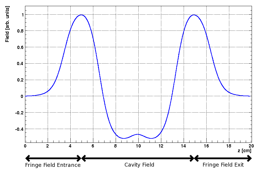
Figure 12.1: The on-axis field of an S-band `TRAVELINGWAVE` structure. The field of a single cavity is shown between its entrance and exit fringe fields.

An example of a 1D traveling-wave field map is shown in Figure 12.1. The map itself is a standing-wave solution for a single accelerating cavity. OPAL-T reconstructs the full traveling-wave tank in three parts:

entrance fringe field,
repeated accelerating-cell region,
exit fringe field.

12.28.1 Fringe fields

The entrance and exit fringe fields are treated as standing-wave regions: \[ \begin{aligned} \mathbf{E}_{\mathrm{entrance}}(\mathbf{r},t) &= \mathbf{E}_{\mathrm{from\,map}}(\mathbf{r})\,\mathrm{VOLT}\, \cos\!\bigl(2\pi\,\mathrm{FREQ}\,t + \phi_{\mathrm{entrance}}\bigr), \\\\ \mathbf{E}_{\mathrm{exit}}(\mathbf{r},t) &= \mathbf{E}_{\mathrm{from\,map}}(\mathbf{r})\,\mathrm{VOLT}\, \cos\!\bigl(2\pi\,\mathrm{FREQ}\,t + \phi_{\mathrm{exit}}\bigr). \end{aligned} \] Here VOLT and FREQ are the element amplitude and frequency, the entrance phase is \phi_{entrance} = \mathrm{LAG}, and the exit phase is determined internally from LAG and NUMCELLS.

12.28.2 Reconstructed body field

The field of the accelerating structure body is reconstructed from the central part of the standing-wave map by superposition: \[ \begin{aligned} \mathbf{E}(\mathbf{r},t) = \frac{\mathrm{VOLT}}{\sin(2\pi\,\mathrm{MODE})} \Bigl[ &\mathbf{E}_{\mathrm{from\,map}}(x,y,z) \cos\!\bigl(2\pi\,\mathrm{FREQ}\,t + \mathrm{LAG} + \tfrac{\pi}{2}\,\mathrm{MODE}\bigr) \\\\ +&\mathbf{E}_{\mathrm{from\,map}}(x,y,z+d) \cos\!\bigl(2\pi\,\mathrm{FREQ}\,t + \mathrm{LAG} + \tfrac{3\pi}{2}\,\mathrm{MODE}\bigr) \Bigr]. \end{aligned} \] The cell spacing is \[ d = \lambda\,\mathrm{MODE}, \] where MODE is expressed in units of 2π. When the longitudinal coordinate advances past the end of the available map interval, OPAL-T subtracts an integer number of cavity wavelengths until the position falls back inside the repeated-cell range.

The legacy model therefore treats the entry and exit half cells through the standing-wave fringe fields and the interior through a repeated-cell traveling wave assembled from the same on-axis map.

The element attributes are:

label: TRAVELINGWAVE, APERTURE=real-vector, L=real,
       VOLT=real, LAG=real, FMAPFN=string,
       ELEMEDGE=real, FREQ=real, NUMCELLS=integer,
       MODE=real;

L: cavity length. In OPAL-T the effective structure length is reconstructed from the field map and NUMCELLS, so L is not the primary geometric input.
VOLT: peak RF voltage. The accelerating phase is again expressed by LAG.
LAG: phase lag in rad. In OPAL-T this is normally defined relative to the phase that maximizes energy gain of the reference particle, as determined by the auto-phasing algorithm.
DLAG: phase-lag error in rad.
FMAPFN: field map in T7 format.
FREQ: traveling-wave frequency in MHz. As for RFCAVITY, OPAL-T warns when this differs from the frequency declared in the field map, and the map value takes precedence.
NUMCELLS: number of accelerating cells, excluding entry and exit half-cell fringes.
MODE: mode in units of 2π; for example 1/3 stands for a 2π/3 structure.
FAST: if TRUE and the field map is 1D, OPAL-T builds a 2D interpolation map and avoids an FFT-based evaluation on every particle and every step.
APVETO: disable auto-phasing for this structure and use the user-supplied LAG directly at the arrival time of the reference particle at the field boundary.

The traveling-wave model requires the particle momentum P and charge CHARGE to be defined on the relevant optics command before the structure is used.

Example:

lrf0: TRAVELINGWAVE, L=0.0253, VOLT=14.750,
      NUMCELLS=40, ELEMEDGE=2.73066,
      FMAPFN="INLB-02-RAC.Ez", MODE=1/3,
      FREQ=1498.956, LAG=248.0/360.0;

12.29 Monitor

A MONITOR detects all particles passing it and writes the position, momentum, and time of impact into an H5hut file. It always has an effective length of 1 cm, consisting of a 0.5 cm drift, the monitor of zero length, and another 0.5 cm drift. This prevents OPAL-T from missing particles.

The positions of the particles on the monitor are interpolated from the current position and momentum one step before they would pass the monitor.

OUTFN: file name into which the monitor writes the collected data.

If TYPE=TEMPORAL, the data of all particles are written when the reference particle hits the monitor.

12.30 Collimators

Four collimator families exist in the legacy manual:

ECOLLIMATOR: elliptic aperture
RCOLLIMATOR: rectangular aperture
FLEXIBLECOLLIMATOR: arbitrary aperture description
CCOLLIMATOR: cyclotron-specific radial rectangular collimator

The common OPAL-T beamline syntax is:

label: ECOLLIMATOR, TYPE=string, APERTURE=real-vector,
       L=real, XSIZE=real, YSIZE=real;

label: RCOLLIMATOR, TYPE=string, APERTURE=real-vector,
       L=real, XSIZE=real, YSIZE=real;

label: FLEXIBLECOLLIMATOR, APERTURE=real-vector,
       L=real, DESCRIPTION=string, FNAME=string, OUTFN=string;

Common attributes:

OUTFN: file name for lost-particle output. If omitted, the element label is used. The output is written as H5hut, or ASCII when ASCIIDUMP is enabled.
PARTICLEMATTERINTERACTION: activates scattering and energy-loss modeling when configured.

12.30.1 OPAL-T mode

Optically, a collimator behaves like a drift space, but during tracking it also introduces an aperture limit. The aperture is checked at the entrance, and if the collimator has nonzero length it is also checked at the exit and at every timestep.

XSIZE: horizontal half-aperture in m.
YSIZE: vertical half-aperture in m.

For ECOLLIMATOR, the values are ellipse half-axes; for RCOLLIMATOR, they are rectangle half-widths.

Example:

Col: ECOLLIMATOR, L=1.0E-3, ELEMEDGE=3.0E-3, XSIZE=5.0E-4,
     YSIZE=5.0E-4, OUTFN="Coll.h5";

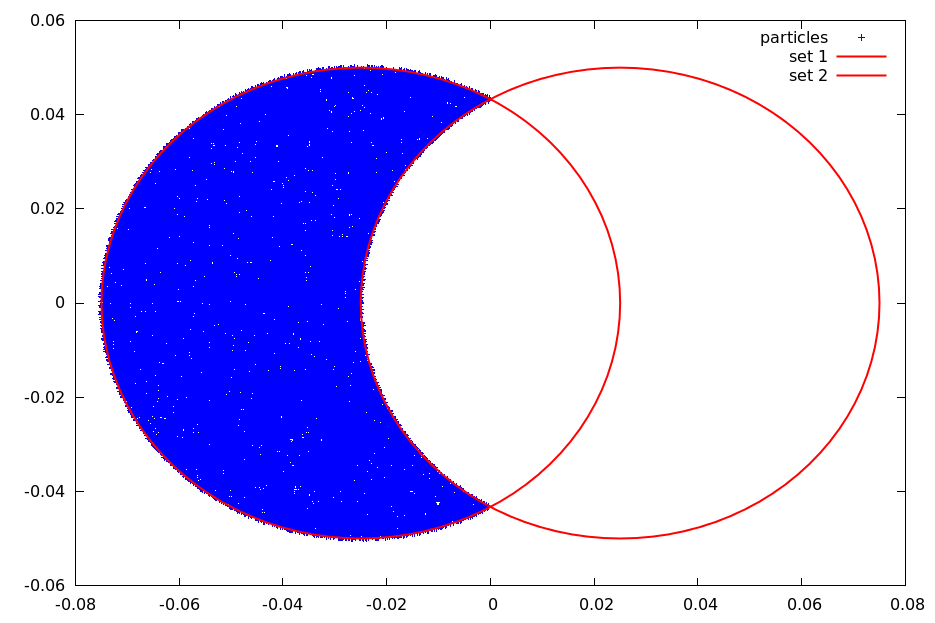
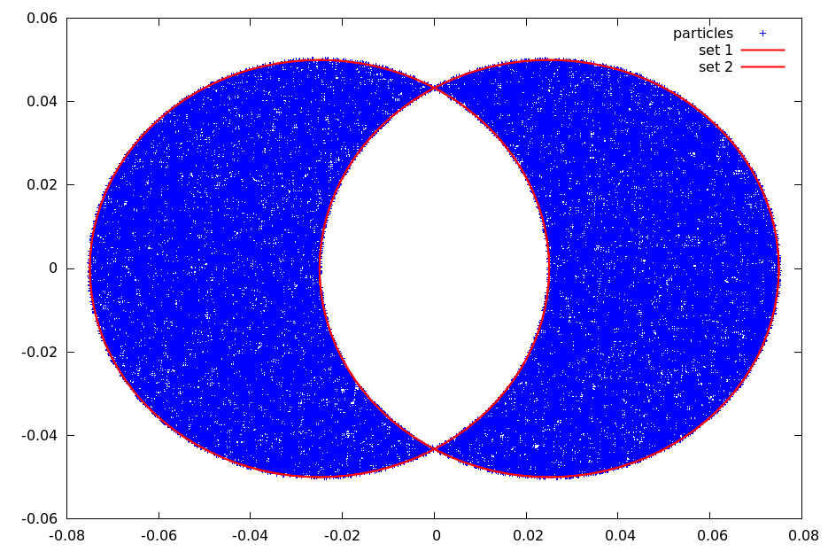
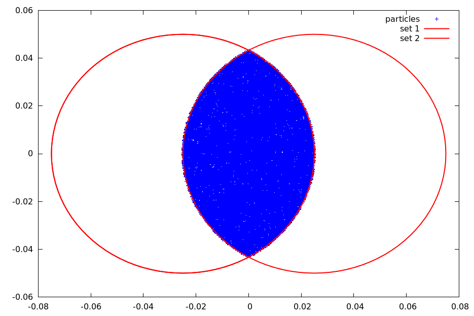
FLEXIBLECOLLIMATOR extends this with a small shape-description language. The supported primitive and composition commands are:

rectangle(width, height): rectangle centered at the origin.
ellipse(width, height): ellipse centered at the origin.
polygon(x0, y0; x1, y1; ...; xN, yN): polygon whose final point is implicitly connected back to the first point. The polygon is triangulated internally, so self-crossing edges are not allowed.
mask('filename.pbm', width, height): black-and-white PBM bitmap mask. White pixels stop particles.
translate(command, shiftx, shifty): translate a shape by (shiftx, shifty).
rotate(command, angle): rotate a shape about the origin.
union(command1, command2, ...): union of several shape definitions.
difference(command1, command2): particles pass command1 but not command2.
symmetric_difference(command1, command2): particles pass either command but not both at the same time.
intersection(command1, command2): particles pass both commands simultaneously.
repeat(command, N, shiftx, shifty): repeat a shape N times with a translational offset.
repeat(command, N, angle): repeat a shape N times with successive rotation.

Figure 12.2: Illustration of a difference between two circles.

Figure 12.3: Illustration of a symmetric difference between two circles.

Figure 12.4: Illustration of an intersection between two circles.

The expression language supports the following constants and functions:

Constants and functions	Constants and functions	Constants and functions	Constants and functions
`e`	`pi`	`abs(x)`	`acos(x)`
`acosh(x)`	`asin(x)`	`asinh(x)`	`atan(x)`
`atanh(x)`	`cbrt(x)`	`ceil(x)`	`cos(x)`
`cosh(x)`	`deg2rad(x)`	`erf(x)`	`erfc(x)`
`exp(x)`	`exp2(x)`	`floor(x)`	`isinf(x)`
`isnan(x)`	`log(x)`	`log2(x)`	`log10(x)`
`rad2deg(x)`	`round(x)`	`sgn(x)`	`sin(x)`
`sinh(x)`	`sqrt(x)`	`tan(x)`	`tanh(x)`
`tgamma(x)`	`atan2(y,x)`	`max(x,y)`	`min(x,y)`
`pow(x,n)`

A simple elliptic collimator can be described by:

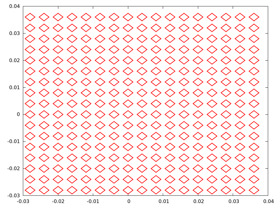
ellipse(0.04, 0.03)

A regular pepper-pot with rectangular holes can be described by:

Figure 12.5: Pepper-pot with rectangular holes.

In FLEXIBLECOLLIMATOR, the hole description can be supplied directly through DESCRIPTION or through an external file specified by FNAME. The external file form is the one that allows comments and line breaks.

12.31 Correctors

Three types of correctors are available:

HKICKER: horizontal corrector
VKICKER: vertical corrector
KICKER: combined horizontal and vertical corrector

They are defined as:

label: HKICKER, TYPE=string, APERTURE=real-vector,
      L=real, KICK=real;
label: VKICKER, TYPE=string, APERTURE=real-vector,
      L=real, KICK=real;
label: KICKER, TYPE=string, APERTURE=real-vector,
      L=real, HKICK=real, VKICK=real;

Attributes:

KICK: kick angle in rad for HKICKER or VKICKER.
HKICK, VKICK: horizontal and vertical kick angles for KICKER.
DESIGNENERGY: if set, fixes the magnetic field magnitude using the given design energy in MeV and the requested kick angle.

A positive kick increases \(p_x\) or \(p_y\) respectively.

Examples:

HK1: HKICKER, KICK=0.001;
VK3: VKICKER, KICK=0.0005;
KHV: KICKER,  HKICK=0.001, VKICK=0.0005;

Correctors do not change the reference trajectory. Otherwise they are implemented like RBEND with E1 = 0 and without fringe fields.

12.32 Bending Magnets

Legacy OPAL supports four bend families:

RBEND for rectangular bends in OPAL-T
RBEND3D for rectangular bends with field-map support in OPAL-T
SBEND for sector bends in OPAL-T

RBEND and SBEND share the same basic dipole semantics but differ in their reference geometry. RBEND has parallel pole faces and an exit angle fixed by ANGLE - E1; SBEND uses a sector reference arc and supports independent entrance and exit edge angles.

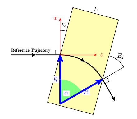
Figure 12.6: Rectangular bend geometry with positive bend angle and positive entrance edge angle.

12.32.1 `RBEND`

Key attributes are:

L: physical magnet length
GAP: full vertical gap
HAPERT: non-bend-plane aperture
ANGLE: bend angle in rad
K0, K0S: normal and skew dipole field amplitudes in T
E1: entrance edge angle
DESIGNENERGY: reference-particle energy in MeV
FMAPFN: fringe-field map, typically 1DProfile1

If ANGLE is set, it overrides K0 and OPAL adjusts the field strength to bend the design particle through the requested angle.

12.32.2 `RBEND3D`

RBEND3D keeps the rectangular bend geometry but uses explicit field-map support for the field model. The input attributes follow the same geometric meaning as RBEND, and the entrance/exit pole-face interpretation stays the same.

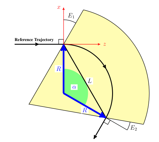
Figure 12.7: Sector bend geometry with independent entrance and exit edge angles.

12.32.3 `SBEND`

SBEND is the sector-bend version. The main difference is the interpretation of L: it is the chord length of the bend reference arc, \[ L = 2 R \sin(\alpha/2) \] and the element has both E1 and E2 as independent edge angles. Very large bend angles are possible, but once the entrance and exit fringe regions begin to overlap, the approximation becomes unreliable.

12.32.4 Bend setup rules in OPAL-T

The original manual emphasizes the following practical points:

Internally OPAL-T treats all bends as positive bends in the local reference frame and then uses ROTATION to orient them in the laboratory transverse plane.
If ANGLE is nonzero, K0 and K0S are ignored.
When ANGLE is used to define the bend strength, the actual beam bend still depends on whether the bunch energy matches DESIGNENERGY.
The hard-edge geometry defines the ideal reference trajectory, while the FMAPFN field map defines the soft-edge magnet seen by tracked particles.
If the default field map 1DPROFILE1-DEFAULT is used, OPAL shifts the fringe-field origins so that the effective length of the soft-edge magnet matches the ideal hard-edge reference bend.

12.32.5 `RBEND` and `SBEND` examples

A simple RBEND driven by ANGLE and the default fringe-field map is:

Bend: RBEND, ANGLE = 30.0 * Pi / 180.0,
      FMAPFN = "1DPROFILE1-DEFAULT",
      ELEMEDGE = 0.25,
      DESIGNENERGY = 10.0E6,
      L = 0.5, GAP = 0.02;

For an electron design beam this produces a 30 degree positive bend, a 1 m reference radius, and a field amplitude of about -0.0350195 T. The important part of the diagnostic output is the final fringe-field integration report, which tells the user the actual bend angle of the reference particle through the soft-edge magnet.

The same bend can be defined through K0 instead of ANGLE:

Bend: RBEND, K0 = -0.0350195,
      FMAPFN = "1DPROFILE1-DEFAULT",
      ELEMEDGE = 0.25,
      DESIGNENERGY = 10.0E6,
      L = 0.5, GAP = 0.02;

To numerical precision this reproduces the same geometry and field.

To bend in the opposite direction, the legacy manual gives four equivalent patterns:

Bend: RBEND, ANGLE = -30.0 * Pi / 180.0,
             FMAPFN = "1DPROFILE1-DEFAULT",
             ELEMEDGE = 0.25,
             DESIGNENERGY = 10.0E6,
             L = 0.5, GAP = 0.02;

Bend: RBEND, ANGLE = 30.0 * Pi / 180.0,
             FMAPFN = "1DPROFILE1-DEFAULT",
             ELEMEDGE = 0.25,
             DESIGNENERGY = 10.0E6,
             L = 0.5, GAP = 0.02,
             ROTATION = Pi;

Bend: RBEND, K0 = 0.0350195,
             FMAPFN = "1DPROFILE1-DEFAULT",
             ELEMEDGE = 0.25,
             DESIGNENERGY = 10.0E6,
             L = 0.5, GAP = 0.02;

Bend: RBEND, K0 = -0.0350195,
             FMAPFN = "1DPROFILE1-DEFAULT",
             ELEMEDGE = 0.25,
             DESIGNENERGY = 10.0E6,
             L = 0.5, GAP = 0.02,
             ROTATION = Pi;

The recommended style is to define the bend in the positive reference orientation and then use ROTATION to place it elsewhere in the transverse plane.

A representative four-dipole chicane setup is:

Bend1: RBEND, ANGLE = 20.0 * Pi / 180.0,
              E1 = 0.0,
              FMAPFN = "1DPROFILE1-DEFAULT",
              ELEMEDGE = 0.25,
              DESIGNENERGY = 10.0E6,
              L = 0.25,
              GAP = 0.02,
              ROTATION = Pi;

Bend2: RBEND, ANGLE = 20.0 * Pi / 180.0,
              E1 = 20.0 * Pi / 180.0,
              FMAPFN = "1DPROFILE1-DEFAULT",
              ELEMEDGE = 1.0,
              DESIGNENERGY = 10.0E6,
              L = 0.25,
              GAP = 0.02,
              ROTATION = 0.0;

Bend3: RBEND, ANGLE = 20.0 * Pi / 180.0,
              E1 = 0.0,
              FMAPFN = "1DPROFILE1-DEFAULT",
              ELEMEDGE = 1.5,
              DESIGNENERGY = 10.0E6,
              L = 0.25,
              GAP = 0.02,
              ROTATION = 0.0;

Bend4: RBEND, ANGLE = 20.0 * Pi / 180.0,
              E1 = 20.0 * Pi / 180.0,
              FMAPFN = "1DPROFILE1-DEFAULT",
              ELEMEDGE = 2.25,
              DESIGNENERGY = 10.0E6,
              L = 0.25,
              GAP = 0.02,
              ROTATION = Pi;

SBEND can be used in the same role once L, E1, and E2 are interpreted using the sector-bend geometry.

12.32.6 Custom `1DProfile1` bend maps

The source manual distinguishes two 1DProfile1 usage modes:

the map defines both the fringe fields and the magnet length,
the map defines only the fringe fields and the element L defines the body length.

In the first mode, a custom map can define an SBEND without supplying L in order to preserve the exit fringe placement:

1DProfile1 1 1 2.0
 -10.0  0.0  10.0 1
  15.0  25.0 35.0 1
  0.00000E+00
  2.00000E+00
  0.00000E+00
  2.00000E+00

Bend: SBEND, ANGLE = 60.0 * Pi / 180.0,
             E1 = -10.0 * Pi / 180.0,
             E2 = 20.0 * Pi / 180.0,
             FMAPFN = "TEST-MAP.T7",
             ELEMEDGE = 0.25,
             DESIGNENERGY = 10.0E6,
             GAP = 0.02;

In the second mode, the field map contains only the entrance and exit fringe profiles and the magnet body is set by L:

1DProfile1 1 1 2.0
 -10.0  0.0  10.0 1
 -10.0  0.0  10.0 1
  0.00000E+00
  2.00000E+00
  0.00000E+00
  2.00000E+00

Bend: SBEND, ANGLE = 60.0 * Pi / 180.0,
             E1 = -10.0 * Pi / 180.0,
             E2 = 20.0 * Pi / 180.0,
             FMAPFN = "TEST-MAP.T7",
             ELEMEDGE = 0.25,
             DESIGNENERGY = 10.0E6,
             L = 0.25,
             GAP = 0.02;

With ANGLE, OPAL adjusts the field amplitude so that the reference particle is bent by the requested amount after the fringe fields are included. With K0, that compensation is not automatic:

Bend: SBEND, K0 = -0.1400778,
             E1 = -10.0 * Pi / 180.0,
             E2 = 20.0 * Pi / 180.0,
             FMAPFN = "TEST-MAP.T7",
             ELEMEDGE = 0.25,
             DESIGNENERGY = 10.0E6,
             L = 0.25,
             GAP = 0.02;

In the original example this produces a small bend mismatch because the soft-edge effective length no longer matches the ideal hard-edge reference magnet. The manual then corrects this by moving the entrance and exit Enge origins outward by 0.03026 mm:

1DProfile1 1 1 2.0
 -10.0  -0.03026  10.0 1
 -10.0   0.03026  10.0 1
  0.00000E+00
  2.00000E+00
  0.00000E+00
  2.00000E+00

This increases the effective magnet length until the final tracked bend of the reference particle matches the desired 60 degree design bend again.

12.32.7 Bend fields from `1DProfile1`

For RBEND and SBEND, OPAL-T divides the field into three regions:

entrance fringe field
central field region
exit fringe field

The fringe regions are modeled from the 1DProfile1 Enge functions associated with FMAPFN.

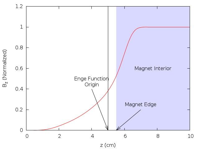
Figure 12.8: Entrance fringe field profile corresponding to the default Enge parameters.

The Enge function is \[ F(z) = \frac{1}{1 + e^{\sum_{n=0}^{N_{\mathrm{order}}} c_n (z/D)^n}} \] where D is the full magnet gap, N_order is the Enge order, and z is the perpendicular distance from the chosen fringe-field origin to the magnet face.

For a positive bend OPAL-T works with:

B_0: dipole field amplitude,
R: bend radius,
n = -(R/B_y)(\partial B_y/\partial x): field index set from K1,
F(\Delta_z): the entrance, central, or exit Enge profile depending on the particle position.

The transverse-local coordinates are:

y: vertical offset from the magnet mid-plane,
\Delta_x: perpendicular distance from the reference trajectory in the bend plane,
\Delta_z: perpendicular distance from the entrance or exit fringe-field origin.

Starting from \[ \nabla \cdot \vec{B} = 0, \qquad \nabla \times \vec{B} = 0, \] and defining \[ F' = \frac{dF}{dz}, \qquad F'' = \frac{d^2F}{dz^2}, \qquad F''' = \frac{d^3F}{dz^3}, \] one may write the exact off-axis field in terms of \[ \kappa(\Delta_z) = \sqrt{\frac{n^2}{R^2} + \frac{F''(\Delta_z)}{F(\Delta_z)}}. \] Then \[ \begin{aligned} B_x(\Delta_x,y,\Delta_z) &= -B_0 \frac{n}{R} e^{-n\Delta_x/R} \frac{F(\Delta_z)}{\kappa(\Delta_z)} \sin\!\bigl(\kappa(\Delta_z)y\bigr), \\\\ B_y(\Delta_x,y,\Delta_z) &= B_0 e^{-n\Delta_x/R} \cos\!\bigl(\kappa(\Delta_z)y\bigr) F(\Delta_z), \\\\ B_z(\Delta_x,y,\Delta_z) &= B_0 e^{-n\Delta_x/R} \Biggl[ \frac{F'\!(\Delta_z)}{\kappa(\Delta_z)}\sin\!\bigl(\kappa(\Delta_z)y\bigr) - \frac{1}{2\kappa(\Delta_z)} \left(F'''\!(\Delta_z) - \frac{F'\!(\Delta_z)F''\!(\Delta_z)}{F(\Delta_z)}\right) \left( \frac{\sin\!\bigl(\kappa(\Delta_z)y\bigr)}{\kappa(\Delta_z)^2} - y\frac{\cos\!\bigl(\kappa(\Delta_z)y\bigr)}{\kappa(\Delta_z)} \right) \Biggr]. \end{aligned} \] For tracking, OPAL-T uses the small-y expansion up to O(y^2).

In the fringe regions: \[ \begin{aligned} B_x &\approx -B_0 \frac{n}{R} e^{-n\Delta_x/R} y, \\\\ B_y &\approx B_0 e^{-n\Delta_x/R} \left[F(\Delta_z) - \left(\frac{n^2}{R^2}F(\Delta_z) + F''\!(\Delta_z)\right)\frac{y^2}{2}\right], \\\\ B_z &\approx B_0 e^{-n\Delta_x/R} y F'\!(\Delta_z). \end{aligned} \] In the central region: \[ \begin{aligned} B_x &\approx -B_0 \frac{n}{R} e^{-n\Delta_x/R} y, \\\\ B_y &\approx B_0 e^{-n\Delta_x/R}\left(1 - \frac{n^2}{R^2}\frac{y^2}{2}\right), \\\\ B_z &\approx 0. \end{aligned} \] These are the expressions OPAL-T uses internally after it determines whether a particle is in the entrance fringe, body, or exit fringe region.

12.32.8 Default bend field map

When FMAPFN="1DPROFILE1-DEFAULT", OPAL uses built-in Enge coefficients for both the entrance and exit fringe regions. The default map corresponds to a 2 cm gap, which may be overridden by the element GAP attribute.

The coefficients are: \[ \begin{aligned} c_0 &= 0.478959, & c_1 &= 1.911289, & c_2 &= -1.185953, \\ c_3 &= 1.630554, & c_4 &= -1.082657, & c_5 &= 0.318111. \end{aligned} \]

The equivalent explicit 1DProfile1 map is:

1DProfile1 5 5 2.0
 -10.0 0.0 10.0 1
 -10.0 0.0 10.0 1
  0.478959
  1.911289
 -1.185953
  1.630554
 -1.082657
  0.318111
  0.478959
  1.911289
 -1.185953
  1.630554
 -1.082657
  0.318111

12.33 Variable RF Cavities

VARIABLE_RF_CAVITY extends the hard-edge cavity model by making frequency, amplitude, and phase explicit functions of time:

FREQUENCY_MODEL=string, AMPLITUDE_MODEL=string, PHASE_MODEL=string

The field is modeled as \[ E(t) = a(t)\,\sin\!\left(2\pi \int_0^t f(\tau)\,d\tau + \phi(t)\right) \] with no field outside the cavity boundary and no transverse dependence in the hard-edge model.

Important geometry attributes are WIDTH, HEIGHT, and L.

12.33.1 Time-dependence models

POLYNOMIAL_TIME_DEPENDENCE: defines \[ g(t) = p_0 + p_1 t + p_2 t^2 + p_3 t^3, \] either via P0..P3 or a longer COEFFICIENTS array.
SPLINE_TIME_DEPENDENCE: uses tabulated TIMES and VALUES with ORDER=1 or 3.
SINUSOIDAL_TIME_DEPENDENCE: sums one or more sine waves from arrays FREQUENCIES, AMPLITUDES, PHASE_OFFSETS, and DC_OFFSETS.

12.33.2 Soft-edged variable cavities

For soft-edged cavities, VARIABLE_RF_CAVITY_FRINGE_FIELD adds:

CENTRE_LENGTH
END_LENGTH
CAVITY_CENTRE
MAX_ORDER

The intention is to place a full cavity including the central flat-top field region and explicit fringe-field ends. VARIABLE_RF_CAVITY_FRINGE_FIELD is the legacy soft-edge companion of VARIABLE_RF_CAVITY.

Example:

RF_FREQUENCY: POLYNOMIAL_TIME_DEPENDENCE, P0=rf_p0, P1=rf_p1, P2=rf_p2, P3=rf_p3;
RF_AMPLITUDE: POLYNOMIAL_TIME_DEPENDENCE, P0=1.0;
RF_PHASE: POLYNOMIAL_TIME_DEPENDENCE, P0=phi;

HARD_RF_CAVITY: VARIABLE_RF_CAVITY,
                PHASE_MODEL="RF_PHASE", AMPLITUDE_MODEL="RF_AMPLITUDE",
                FREQUENCY_MODEL="RF_FREQUENCY", L=0.100, HEIGHT=0.200, WIDTH=2.000;

SOFT_RF_CAVITY: VARIABLE_RF_CAVITY_FRINGE_FIELD,
                PHASE_MODEL="RF_PHASE", AMPLITUDE_MODEL="RF_AMPLITUDE",
                FREQUENCY_MODEL="RF_FREQUENCY", L=0.200, HEIGHT=0.200, WIDTH=2.000,
                CENTRE_LENGTH=0.1, END_LENGTH=0.01, CAVITY_CENTRE=0.1, MAX_ORDER=4;

12.34 Septum

SEPTUM is a cyclotron-side extraction element. Particles hitting the septum are removed from the bunch and written to the element output file.

Main geometric attributes:

XSTART, XEND
YSTART, YEND
WIDTH

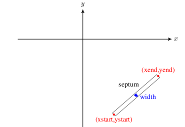
Figure 12.9: Cyclotron `SEPTUM` geometry.

Example:

eec2: SEPTUM, XSTART=4100.0, XEND=4300.0,
      YSTART=-1200.0, YEND=-150.0, WIDTH=0.05;

Lost particles are written to OUTFN.h5 or ASCII when ASCIIDUMP is enabled. ## Probe {#opal-probe}

PROBE records particles crossing a line-like detector while leaving them in the simulation.

Main attributes:

XSTART, XEND
YSTART, YEND
STEP: histogram step size for the associated probe histogram and peak files

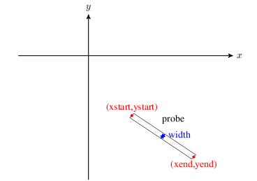
Figure 12.10: Cyclotron `PROBE` geometry.

Example:

prob1: PROBE, XSTART=4166.16, XEND=4250.0,
       YSTART=-1226.85, YEND=-1241.3;

The hit particles are recorded in OUTFN.h5 (or ASCII with ASCIIDUMP). The same crossings are also accumulated into the .hist and .peaks files that mimic measured probe histograms and their derived peak locations. ## Output Plane {#opal-output-plane}

OUTPUTPLANE records particles crossing a plane in space. Unlike PROBE, the plane can be defined either by a probe-style segment or by an explicit center and normal.

Two placement styles are available:

PROBE: uses XSTART, XEND, YSTART, YEND
CENTRE_NORMAL: uses CENTRE, NORMAL, together with optional WIDTH, HEIGHT, and RADIUS

Additional controls include:

REFERENCE_ALIGNMENT_PARTICLE
TOLERANCE
ALGORITHM = INTERPOLATION | RK4
VERBOSE

In CENTRE_NORMAL mode the plane may realign itself on the first crossing of REFERENCE_ALIGNMENT_PARTICLE so that the plane center and normal follow that reference trajectory.

Example:

outplane1: OUTPUTPLANE, PLACEMENT_STYLE=CENTRE_NORMAL,
           CENTRE={10, 13.5, 0}, NORMAL={1,0,0},
           WIDTH=1.5, HEIGHT=0.8, RADIUS=1,
           ALGORITHM=RK4, VERBOSE=1,
           REFERENCE_ALIGNMENT_PARTICLE=0, OUTFN="FileName.txt";

12.35 Stripper

STRIPPER is the cyclotron extraction element that changes particle charge and mass when a particle hits the stripping foil geometry.

Important attributes are:

XSTART, XEND, YSTART, YEND
OPCHARGE: output charge state
OPMASS: output particle mass
OPYIELD: number of outgoing particles per incoming particle
STOP: if TRUE, stop the particle after stripping

The geometry matches the PROBE-style line segment. The struck particles are always written to the output file, regardless of STOP. The legacy manual also states explicitly that this element changes charge and mass but does not yet model the full microscopic stripping process.

Example:

prob1: STRIPPER, XSTART=4166.16, XEND=4250.0,
                 YSTART=-1226.85, YEND=-1241.3,
                 OPCHARGE=1, OPMASS=PMASS,
                 OPYIELD=2, STOP=FALSE;

12.36 Degrader

DEGRADER is an OPAL-T particle-matter interaction element with an elliptical transverse profile and length L.

Important attributes are:

XSIZE, YSIZE: ellipse axes
PARTICLEMATTERINTERACTION: attach scattering and energy-loss modeling

If no particle-matter interaction handler is attached, particles hitting the degrader are simply recorded and deleted.

Example:

DEGPHYS: PARTICLEMATTERINTERACTION, TYPE=SCATTERING, MATERIAL=GRAPHITE;
DEG1: DEGRADER, L=0.15, ELEMEDGE=0.02, PARTICLEMATTERINTERACTION=DEGPHYS;

12.37 Vacuum

VACUUM represents interactions with residual gas and, when configured, the associated stripping physics. When an interaction occurs, the particle state at that instant is written out.

MINR, and MAXR limits. In OPAL-T it is described by the usual L and ELEMEDGE placement parameters.

Important attributes are:

PRESSURE: average residual-gas pressure in mbar
TEMPERATURE: gas temperature in K
GAS = H2 | AIR
STOP: whether the interacting particle is deleted immediately
PARTICLEMATTERINTERACTION

Cyclotron mode additionally supports a pressure map through:

PMAPFN: mid-plane pressure-map file
PSCALE: scale factor applied to that map

If PMAPFN is supplied, PRESSURE acts as the default value outside the map extent. For stripping studies, PARTICLEMATTERINTERACTION should usually point to a handler with TYPE=BEAMSTRIPPING.

Example:

bstp_phys: PARTICLEMATTERINTERACTION, TYPE=BEAMSTRIPPING;
vac: VACUUM, PRESSURE=1E-8, TEMPERATURE=300,
     GAS=H2, STOP=true, PARTICLEMATTERINTERACTION=bstp_phys;

The particles stripped in the residual gas are written to the configured output file regardless of the value of STOP. ## Undulator {#opal-undulator}

UNDULATOR couples the beamline to OPAL’s full-wave FEL solver path. In the legacy implementation the field solve switches from Poisson to a Finite-Difference Time-Domain full-wave model while the bunch traverses the undulator. This path relies on the external MITHRA library.

To use this feature, OPAL must be built with MITHRA support:

install the MITHRA library,
set MITHRA_PREFIX to its installation path,
configure OPAL with -DENABLE_OPAL_FEL=yes.

When the head of the bunch crosses the undulator start, the solver switches to full-wave and returns to Poisson once the bunch has passed the undulator and its fringe fields.

The effective undulator length is determined by the number of periods and the built-in fringe extent, \[ L = N\lambda + 2\,\mathrm{fringe}, \qquad \mathrm{fringe} = 2\lambda, \] so there is no separate user-supplied L parameter.

The idealized planar-undulator field is \[ B_x = B_0\cosh(kr)\sin(kz)\cos(\alpha), \] \[ B_y = B_0\cosh(kr)\sin(kz)\sin(\alpha), \] \[ B_z = B_0\sinh(kr)\cos(kz), \] with \(k = 2\pi/\lambda\) and polarization angle \(\alpha\).

Important attributes are:

K: undulator strength parameter
LAMBDA: undulator period
NUMPERIODS: number of periods
ANGLE: polarization angle
MESHLENGTH: computational-domain size in the moving bunch frame
MESHRESOLUTION: computational-grid spacing
DTBUNCH: particle update timestep
TRUNORDER: absorbing-boundary truncation order
TOTALTIME: total full-wave simulation time
FNAME: optional job/output description file for the full-wave solver

Example:

UND: UNDULATOR, ELEMEDGE = 44.0e-2, K = 10.81, LAMBDA = 8.5e-2, NUMPERIODS = 10, ANGLE = PI/2,
     MESHLENGTH = { 12e-3, 12e-3, 4e-3 }, MESHRESOLUTION = { 1e-5, 1e-5, 8e-6},
     FNAME = "wiggler_sims_July_2020/mithra_output.job";

12.1 Common element syntax

12.2 DRIFT

12.3 CONSTANTEFIELDCAVITY

12.4 QUADRUPOLE

12.5 MULTIPOLE

12.6 MULTIPOLET

12.7 SOLENOID

12.8 RFCAVITY

12.9 TRAVELINGWAVE

12.10 LASER

12.11 MONITOR

12.12 MARKER

12.13 PROBE

12.14 RBEND and SBEND

12.15 VERTICALFFAMAGNET

12.16 VARIABLE_RF_CAVITY

12.16.1 Time-dependence definitions

12.17 Current limitations

12.18 Element Input Format

12.19 Common Attributes for All Elements

12.20 Drift Spaces

12.21 Quadrupole

12.22 Sextupole

12.23 Octupole

12.24 General Multipole

12.25 General Multipole With Fringe Field Model

12.26 Solenoid

12.27 RF Cavities

12.27.1 OPAL-T mode

12.28 Traveling Wave Structure

12.28.1 Fringe fields

12.28.2 Reconstructed body field

12.29 Monitor

12.30 Collimators

12.30.1 OPAL-T mode

12.31 Correctors

12.32 Bending Magnets

12.32.1 RBEND

12.32.2 RBEND3D

12.32.3 SBEND

12.32.4 Bend setup rules in OPAL-T

12.32.5 RBEND and SBEND examples

12.32.6 Custom 1DProfile1 bend maps

12.32.7 Bend fields from 1DProfile1

12.32.8 Default bend field map

12.33 Variable RF Cavities

12.33.1 Time-dependence models

12.33.2 Soft-edged variable cavities

12.34 Septum

12.35 Stripper

12.36 Degrader

12.37 Vacuum

12.2 `DRIFT`

12.3 `CONSTANTEFIELDCAVITY`

12.4 `QUADRUPOLE`

12.5 `MULTIPOLE`

12.6 `MULTIPOLET`

12.7 `SOLENOID`

12.8 `RFCAVITY`

12.9 `TRAVELINGWAVE`

12.10 `LASER`

12.11 `MONITOR`

12.12 `MARKER`

12.13 `PROBE`

12.14 `RBEND` and `SBEND`

12.15 `VERTICALFFAMAGNET`

12.16 `VARIABLE_RF_CAVITY`

12.32.1 `RBEND`

12.32.2 `RBEND3D`

12.32.3 `SBEND`

12.32.5 `RBEND` and `SBEND` examples

12.32.6 Custom `1DProfile1` bend maps

12.32.7 Bend fields from `1DProfile1`