37 Field Solver Physics
This chapter is the physics-level counterpart to the Field Solver user guide. The user guide documents input choices and current runtime behavior; this chapter will derive the model, state its approximations, and collect numerical validation.
The headings below define the intended scope. They deliberately contain only short writing prompts so that equations and claims can be added after they are checked against the implementation and benchmark cases.
37.1 Scope and notation
Define the charge, field, coordinate, unit, and sign conventions used throughout the chapter. State which parts apply to all solvers and which are specific to space charge.
37.2 Governing electrostatic model
State the quasi-static approximation and the physical problem solved in the selected bunch frame.
37.2.1 Poisson equation
Introduce the source term, potential, electric field, and boundary data.
37.2.2 Self-field force
Connect the solved fields to the force applied by the tracker, including any frame transformation required before the particle push.
37.3 Particle-mesh discretization
Describe the complete particle-in-cell cycle and identify the discrete quantities that live on particles and on the mesh.
37.3.1 Charge deposition
Specify the particle shape, weighting rule, normalization, and treatment of ghost cells.
37.3.2 Mesh solve
Define the discrete Poisson operator or convolution used by each solver family.
37.3.3 Field reconstruction and interpolation
Explain how the electric field is reconstructed and interpolated back to particle positions.
37.4 Frames and relativistic transformations
For binned space charge, OPALX first constructs a beam-aligned frame whose origin follows the bunch and whose longitudinal axis is parallel to the mean momentum. Let \(Q\) denote its orthogonal rotation. Particle coordinates entering the binned calculation are
\[ \mathbf r'_i=Q(\mathbf r_i-\mathbf r_0), \qquad \mathbf p'_i=Q\mathbf p_i. \]
Both transformations are required: using \(\mathbf r'_i\) with unrotated \(\mathbf p_i\) mixes coordinate systems in bin selection, mean-bin momentum, and the field transformation. Because \(Q\) is orthogonal, \(|\mathbf p'_i|=|\mathbf p_i|\) and \(\gamma_i=\sqrt{1+|\mathbf p_i|^2}\) is unchanged. After gathering, positions, momenta, and electromagnetic fields are rotated back to the tracking frame.
37.5 Boundary conditions and Green functions
Define each boundary-value problem independently of its input syntax.
37.5.1 Periodic boundaries
Describe the periodic domain, compatibility conditions, and zero-mode handling.
37.5.2 Open boundaries
Derive the free-space Green-function convolution and doubled-domain method.
37.5.3 Dirichlet and image-charge boundaries
Explain explicit image-charge and shifted-Green constructions, including the geometries and assumptions for which they are valid.
37.6 Solver formulations
Relate the mathematical problem to the available numerical backends.
37.6.1 Periodic FFT solver
Document the spectral formulation, differentiation, normalization, and parallel decomposition.
37.6.2 Hockney open-boundary solver
Document domain doubling, kernel sampling, padding, and extraction of the physical-domain result.
37.6.3 Iterative solvers
Reserve this subsection for the operator, convergence criterion, preconditioning, and supported boundary conditions once an iterative backend is production-ready.
37.7 Binned rest-frame space charge
For each populated bin \(b\), OPALX computes the mean normalized momentum \(\mathbf p_b\) and a representative Lorentz factor \(\gamma_b\). The longitudinal mesh spacing is stretched by \(\gamma_b\), charge is deposited and solved in the approximate bin rest frame, and the gathered electric field \(\mathbf E'_b\) is transformed back according to
\[ \mathbf E_b=\gamma_b\mathbf E'_b -(\gamma_b-1)(\mathbf E'_b\cdot\widehat{\mathbf v}_b)\widehat{\mathbf v}_b, \qquad \mathbf B_b=\frac{\gamma_b}{c^2}\mathbf v_b\times\mathbf E'_b, \]
where \(\mathbf v_b=c\mathbf p_b/\gamma_b\). Contributions from all populated bins are accumulated before the particle push. One explicit bin applies a single common boost to the bunch; multiple bins approximate a longitudinally varying velocity distribution.
37.8 Emission and conducting boundaries
Describe how emission time, cathode geometry, image charges, and activation of space charge interact.
37.9 Numerical accuracy and convergence
Collect the error sources that should be varied in convergence studies.
37.9.1 Mesh resolution
Define spatial refinement studies and expected convergence observables.
37.9.2 Particle noise and deposition order
Separate sampling noise from mesh and solver error.
37.9.3 Time-step coupling
The particle step is a drift–kick–drift composition. OPALX provides two self-field sampling conventions while retaining the same Boris kick and external-field evaluation at the midpoint.
For the default midpoint convention,
\[ \mathbf r_{n+1/2}=D_{\Delta t/2}(\mathbf r_n,\mathbf p_n),\qquad (\mathbf E_{\mathrm{sc}},\mathbf B_{\mathrm{sc}})_{n+1/2} =\mathcal S(\mathbf r_{n+1/2},\mathbf p_n), \]
followed by the full Boris momentum kick and the second half drift. The historical pre-step convention instead evaluates
\[ (\mathbf E_{\mathrm{sc}},\mathbf B_{\mathrm{sc}})_n =\mathcal S(\mathbf r_n,\mathbf p_n) \]
before the first half drift. Those gathered fields remain attached to their particles through that drift and are combined with midpoint external fields. The input choices are SCFIELDUPDATE="MIDPOINT" and "PRESTEP"; changing the choice changes the temporal discretization and therefore requires a new timestep-convergence study.
37.10 Domain decomposition and load balancing
Explain which mathematical data are repartitioned and why the field, particle, and solver state must be refreshed in a defined order.
37.11 Current implementation architecture
The following diagram is retained as TikZ source for PDF output. HTML uses a small generated PNG of the same source so the page does not depend on a browser-side TikZ renderer.
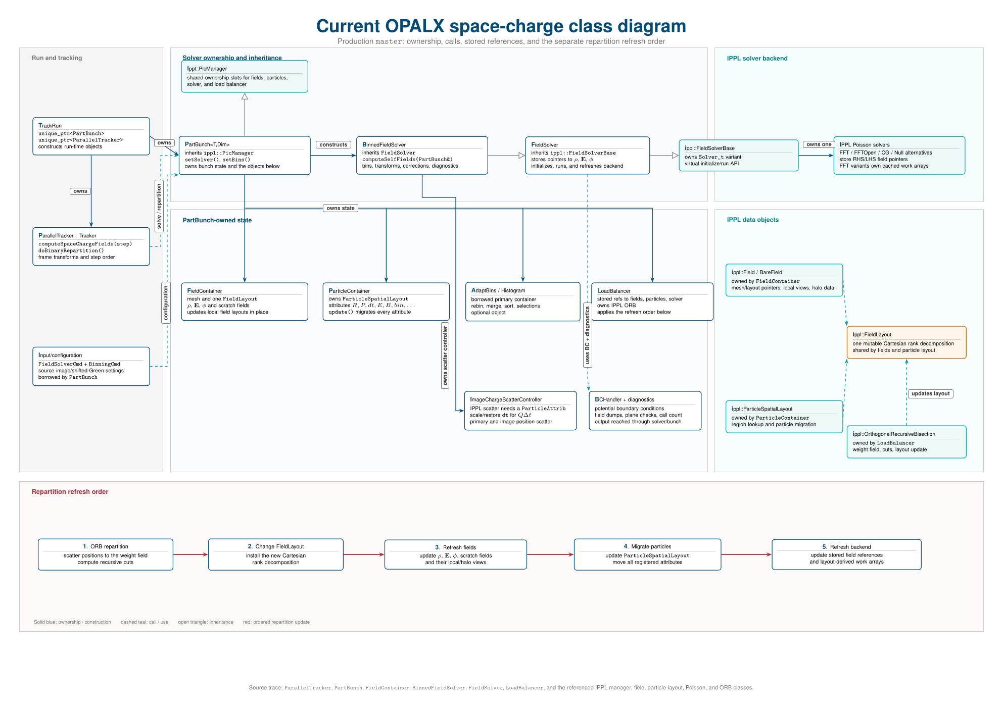
figures/current-space-charge-class-diagram.tex.
37.12 Verification and benchmarks
A one-turn coasting benchmark compared OPALX with OPAL 2022.1 at 72 MeV using a 2 mA proton bunch, 262144 macroparticles, a \(32^3\) open mesh, one momentum bin, GREENSF=STANDARD, and the common timestep \(1.645278052\times10^{-10}\) s. After applying the common-frame momentum rotation, the endpoint comparison was:
| Observable | OPAL 2022.1 | OPALX | Relative difference |
|---|---|---|---|
| radial RMS size [mm] | 4.608578 | 4.605885 | -0.0584% |
| vertical RMS size [mm] | 4.215521 | 4.217434 | +0.0454% |
| longitudinal RMS size [mm] | 1.980226 | 1.981539 | +0.0663% |
| radial normalized RMS emittance [mm mrad] | 2.793744 | 2.793274 | -0.0168% |
| vertical normalized RMS emittance [mm mrad] | 1.012587 | 1.014261 | +0.1654% |
| longitudinal normalized RMS emittance [mm mrad] | 0.192261 | 0.190979 | -0.6667% |
| RMS energy spread [keV] | 43.354672 | 43.176349 | -0.4113% |
These values establish a cross-code regression point at one discretization; they are not a mesh, particle-number, or timestep-convergence result. A clean comparison of the two SCFIELDUPDATE conventions with the production field reconstruction remains to be added.
37.13 Assumptions and known limitations
Maintain a concise list of model assumptions, unsupported combinations, and known numerical limitations, with links to reproducible investigations.