16  Beam and Distributions

OPALX separates the sampled phase space from its placement in the simulation:

Dist: DISTRIBUTION, TYPE=GAUSS, NPARTDIST=10000,
      SIGMAX=1e-3, SIGMAY=1e-3, SIGMAZ=2e-3,
      SIGMAPX=1e-4, SIGMAPY=1e-4, SIGMAPZ=1e-4;
Source: EMISSIONSOURCE, DISTRIBUTION=Dist;
Sources: EMISSIONSOURCELIST=(Source);
Beam: BEAM, PARTICLE=ELECTRON, PC=0.1, NALLOC=10000,
      BCHARGE=-1e-9, SOURCES=Sources;

The DISTRIBUTION defines the particle sample, EMISSIONSOURCE adds source offsets and timing, EMISSIONSOURCELIST groups sources, and BEAM.SOURCES selects the group. See Beam Definitions for the complete BEAM attribute table and its reference-energy rules.

16.1 EMISSIONSOURCE

name: EMISSIONSOURCE, DISTRIBUTION=distribution_name, ...;

Offsets are applied after sampling. Position uses metres, momentum uses dimensionless normalized momentum \(\boldsymbol{p}/mc=\boldsymbol{\beta}\gamma\), and time uses seconds.

Parameter	Default	Meaning and constraints
DISTRIBUTION	required	Previously defined DISTRIBUTION name.
R0X, R0Y, R0Z	0 m	Position offset added to every sampled particle.
P0X, P0Y, P0Z	0	Normalized-momentum offset added after sampling.
T0	0 s	Source start time. For one-shot types, T0 > 0 delays injection.
EMISSIONMODEL	NONE	NONE or ASTRA; availability depends on distribution type.
EKIN	0 eV	Thermal kinetic energy for generated emitted particles; OPALX uses its absolute value.
ZEROFACE_R0Z	FALSE	Apply explicit image-charge Dirichlet correction at \(z=\mathrm{R0Z}\).
SHIFTED_GREENS_FUNCTION	FALSE	Alternative shifted-Green correction; requires an OPEN field solver.
ZEROFACEPLANEDUMP	0	Non-negative integer dump frequency; requires ZEROFACE_R0Z=TRUE.
ZEROFACE_MAXSTEPS	0	Non-negative correction-step limit; 0 means unlimited.

ZEROFACE_R0Z and SHIFTED_GREENS_FUNCTION are mutually exclusive. A run can activate at most one source plane by either method.

For generated emission, NONE adds the momentum corresponding to EKIN in \(+z\). ASTRA samples the forward half-sphere with magnitude

\[ p_{\mathrm{th}}=\sqrt{\left(1+\frac{E_{\mathrm{kin}}}{mc^2}\right)^2-1}, \qquad p_z\geq 0, \]

before adding P0X, P0Y, and P0Z.

16.2 EMISSIONSOURCELIST

Sources: EMISSIONSOURCELIST=(Source1, Source2);

The list is ordered and must contain at least one previously defined EMISSIONSOURCE. Attach it with SOURCES=Sources on BEAM. Several sources may use the same distribution, each with independent offsets and start time.

16.3 DISTRIBUTION

name: DISTRIBUTION, TYPE=distribution_type, ...;

OPALX accepts exactly GAUSS, MULTIVARIATEGAUSS, FLATTOP, OPALFLATTOP, FROMFILE, and EMITTEDFROMFILE.

Available input parameters

Parameter	Default / unit	Used by	Runtime effect
TYPE	required	all	Selects one of the six types above.
NPARTDIST	0, particles	all	Requested macroparticle count. Use a positive integer except where EMITTEDFROMFILE explicitly selects all file records.
FNAME	empty, path	file types	Input particle file. Relative paths are resolved from the OPALX input file.
SIGMAX, SIGMAY, SIGMAZ	0 m	Gaussian types; transverse flat-top types	Spatial widths; flat-top SIGMAX and SIGMAY are ellipse semi-axes.
SIGMAPX, SIGMAPY, SIGMAPZ	0, \(\beta\gamma\)	Gaussian types	RMS normalized-momentum widths.
CORR	empty array	MULTIVARIATEGAUSS	Fifteen off-diagonal correlation coefficients.
SIGMAT	0 s	flat-top types; optional emitted-file window	Default RMS width for both pulse edges.
TPULSEFWHM	0 s	flat-top types; optional emitted-file window	Full pulse width at half maximum.
TRISE, TFALL	0 s	flat-top types; optional emitted-file window	Edge times; a positive value overrides the corresponding SIGMAT.
CUTOFFLONG	3, \(\sigma\)	flat-top types; optional emitted-file window	Truncates both Gaussian pulse edges.
FTOSCAMPLITUDE	0 %	OPALFLATTOP	Sinusoidal modulation amplitude, clamped to 100%.
FTOSCPERIODS	0	OPALFLATTOP	Number of modulation periods across the flat interval.
EMITTED	FALSE	flat-top types; optional emitted-file window	Enables generated time-dependent emission.
EMISSIONSTEPS	100	OPALFLATTOP, EMITTEDFROMFILE	Preferred emission resolution; positive values are rounded up.
CUTOFFX, CUTOFFY	3, \(\sigma\)	none currently	Accepted but currently ignored by active samplers.
CUTOFFPX, CUTOFFPY, CUTOFFPZ	3, \(\sigma\)	none currently	Accepted but currently ignored; Gaussian bounds are fixed internally.
CORRX, CORRY, CORRZ, CORRT	0	none currently	Accepted but currently ignored; use CORR with MULTIVARIATEGAUSS.

Non-file distributions require PC, ENERGY, or GAMMA on BEAM. FROMFILE and EMITTEDFROMFILE contain absolute normalized momenta and reject those three beam-energy attributes.

16.3.1 GAUSS

GAUSS samples independent coordinates. Positions are truncated at the internally fixed \(\pm3\sigma\) bounds and translated so their sampled mean is zero; momenta are unbounded normals around the beam reference momentum.

\[ R_i\sim\mathcal{N}(0,\sigma_{R_i}^2),\qquad P_i\sim\mathcal{N}(\bar P_i,\sigma_{P_i}^2). \]

Use	Parameters
Count	NPARTDIST (positive integer)
Position	SIGMAX, SIGMAY, SIGMAZ
Momentum	SIGMAPX, SIGMAPY, SIGMAPZ
Source	R0*, P0*, T0; EMISSIONMODEL=NONE only

G: DISTRIBUTION, TYPE=GAUSS, NPARTDIST=10000,
   SIGMAX=1e-3, SIGMAY=1e-3, SIGMAZ=2e-3,
   SIGMAPX=1e-4, SIGMAPY=1e-4, SIGMAPZ=2e-4;

With T0 > 0, the complete sample is injected once when a tracker step crosses T0. Named correlations and user-supplied cutoffs do not affect this sampler.

16.3.2 MULTIVARIATEGAUSS

Let

\[ q=(x,p_x,y,p_y,z,p_z)^T,\qquad D=\operatorname{diag}(\sigma_x,\sigma_{p_x},\sigma_y,\sigma_{p_y}, \sigma_z,\sigma_{p_z}). \]

CORR defines a correlation matrix \(C\) and the sampler forms \(\Sigma=DCD=LL^T\), then applies the Cholesky factor \(L\) to independent normal samples. \(C\) must be symmetric positive definite.

Use	Parameters
Count and widths	NPARTDIST, all six SIGMA* values
Coupling	CORR with exactly 15 values
Source	R0*, P0*, T0; EMISSIONMODEL=NONE only

The array is the upper triangle in this order:

(x,px), (x,y), (x,py), (x,z), (x,pz),
(px,y), (px,py), (px,z), (px,pz),
(y,py), (y,z), (y,pz), (py,z), (py,pz), (z,pz)

MG: DISTRIBUTION, TYPE=MULTIVARIATEGAUSS, NPARTDIST=10000,
    SIGMAX=1e-3, SIGMAPX=1e-4,
    SIGMAY=1e-3, SIGMAPY=1e-4,
    SIGMAZ=2e-3, SIGMAPZ=2e-4,
    CORR={0.2,0,0,0,0, 0,0,0,0, 0,0,0, 0,0,0};

Sampling uses internally fixed three-sigma bounds. T0 > 0 produces one delayed injection, as for GAUSS.

16.3.3 FLATTOP

FLATTOP is a time-dependent emitter. Transverse positions are uniform on an ellipse with semi-axes \(a=\mathrm{SIGMAX}\) and \(b=\mathrm{SIGMAY}\):

\[ x=a\sqrt{u}\cos(2\pi v),\qquad y=b\sqrt{u}\sin(2\pi v),\qquad u,v\sim U(0,1). \]

Use	Parameters
Required	NPARTDIST>0, EMITTED=TRUE, SIGMAX, SIGMAY
Pulse	SIGMAT or TRISE/TFALL, TPULSEFWHM, CUTOFFLONG
Source	T0, R0*, P0*, EKIN; EMISSIONMODEL=NONE or ASTRA

For a positive TRISE or TFALL, OPALX converts the corresponding input edge time to an RMS width using

\[ \sigma=\frac{T_{\mathrm{edge}}} {\sqrt{2\ln 10}-\sqrt{2\ln(10/9)}}. \]

With edge widths \(\sigma_r\), \(\sigma_f\) and cutoff \(C\), the flat interval and total emission duration are

\[ T_{\mathrm{flat}}=\max\!\left(0,T_{\mathrm{FWHM}} -\sqrt{2\ln2}(\sigma_r+\sigma_f)\right),\qquad T_{\mathrm{emit}}=C(\sigma_r+\sigma_f)+T_{\mathrm{flat}}. \]

The rate consists of truncated Gaussian rise and fall edges around a constant flat interval. Each tracker step integrates that profile and gives newborn particles a random fractional timestep.

FT: DISTRIBUTION, TYPE=FLATTOP, NPARTDIST=10000, EMITTED=TRUE,
    SIGMAX=1e-3, SIGMAY=1e-3,
    TRISE=0.5e-12, TFALL=0.5e-12,
    TPULSEFWHM=10e-12, CUTOFFLONG=3;

16.3.4 OPALFLATTOP

OPALFLATTOP uses the same transverse and pulse mathematics as FLATTOP, but precomputes a globally sorted inventory of particle birth times. This gives an exact requested inventory and OPAL-compatible pulse centering.

Use	Parameters
Required	All FLATTOP parameters; NPARTDIST>0 and EMITTED=TRUE are enforced
Resolution	EMISSIONSTEPS
Modulation	FTOSCAMPLITUDE, FTOSCPERIODS
Source	T0, R0*, P0*, EKIN; EMISSIONMODEL=NONE or ASTRA

On the flat interval, birth-time density is proportional to

\[ 1+a\sin\!\left(2\pi n\frac{t}{T_{\mathrm{flat}}}\right),\qquad a=\min\!\left(1,\frac{|\mathrm{FTOSCAMPLITUDE}|}{100}\right), \]

where \(n=|\mathrm{FTOSCPERIODS}|\).

OFT: DISTRIBUTION, TYPE=OPALFLATTOP, NPARTDIST=10000, EMITTED=TRUE,
     SIGMAX=1e-3, SIGMAY=1e-3,
     TRISE=0.5e-12, TFALL=0.5e-12,
     TPULSEFWHM=10e-12, CUTOFFLONG=3,
     EMISSIONSTEPS=100, FTOSCAMPLITUDE=5, FTOSCPERIODS=3;

16.3.5 FROMFILE

FROMFILE reads an injected 6D sample. Set a positive NPARTDIST; OPALX uses at most that many records from the beginning of the file.

Use	Parameters
Required	FNAME, positive NPARTDIST
Source	R0*, P0*, T0; EMISSIONMODEL=NONE only
Beam	Omit PC, ENERGY, and GAMMA

The first non-comment line is the declared count, the second is a header, and exactly that many data rows must follow. Header order is arbitrary but must contain x, y, z, px, py, and pz (case-insensitive). Blank lines and lines beginning with # are ignored.

3
x px y py z pz
0.0 0.001 0.0 0.000 0.0 1.2
0.1 0.002 0.0 0.001 0.0 1.2
-0.1 0.000 0.0 -0.001 0.0 1.2

FF: DISTRIBUTION, TYPE=FROMFILE, FNAME="particles.txt", NPARTDIST=3;

Positions are metres and file momenta are absolute \(\beta\gamma\) values. Source offsets are added after reading. T0 > 0 delays the complete file sample to one tracker step.

16.3.6 EMITTEDFROMFILE

EMITTEDFROMFILE reads old-OPAL emitted records and releases them according to their file times.

Use	Parameters
Required	FNAME; NPARTDIST=0 selects all records, otherwise it selects a prefix
Resolution	EMISSIONSTEPS
Optional window	EMITTED=TRUE plus flat-top pulse parameters
Source	R0*, P0*, T0; EMISSIONMODEL=NONE only
Beam	Omit PC, ENERGY, and GAMMA

Rows are positional: x px y py t pz [bin]. The positive-integer bin column is optional. A file may use a leading count and header, or a comment header.

3
x px y py t pz bin
0.0 0.001 0.0 0.000 -2e-12 1.2 1
0.1 0.002 0.0 0.001 -1e-12 1.2 2
-0.1 0.000 0.0 -0.001 0.0 1.2 3

EFF: DISTRIBUTION, TYPE=EMITTEDFROMFILE,
     FNAME="emitted.txt", NPARTDIST=0, EMISSIONSTEPS=100;

Without bins or a configured window, OPALX negates the old-OPAL file times, centres their span, and uses

\[ t_{\mathrm{birth}}=\mathrm{T0}-t_{\mathrm{file}}-t_{\mathrm{centre}}. \]

An enabled flat-top window may replace the inferred span, but it must cover the latest selected file time. Positions and momenta receive the source offsets; the file momenta remain absolute.

16.4 Reproducibility and current limitations

Record the OPALX revision, random seed, NPARTDIST, BEAM.NALLOC, bunch charge, source list, and every referenced file. Keep NALLOC at least as large as the sum of the source distributions’ particle counts.

Current source limitations are deliberate documentation constraints:

• only MULTIVARIATEGAUSS.CORR affects correlations;
• Gaussian cutoff attributes are parsed but sampling uses internal bounds;
• FTOSCAMPLITUDE and FTOSCPERIODS affect only OPALFLATTOP;
• ASTRA is supported only by the generated flat-top emitters; and
• file distributions take momentum from their files, not from BEAM energy.

The DISTRIBUTION command defines how particles are introduced into a simulation. A distribution has a name, a type, and a set of attributes that control its geometry, momentum spread, emission behavior, and optional correlations.

Name: DISTRIBUTION, TYPE = DISTRIBUTION_TYPE,
      ATTRIBUTE1 = ...,
      ATTRIBUTE2 = ...;

The supported distribution types depend on whether you are looking at the legacy OPAL manual path or the current OPALX implementation.

Type	Description
FROMFILE	Read initial particle coordinates from a user-provided text file.
GAUSS	Gaussian distribution in one or more dimensions.
FLATTOP	Hard-edge transverse distribution with flat-top time structure.
BINOMIAL	Binomial family controlled by one shape parameter per axis.
GAUSSMATCHED	Matched Gaussian distribution for cyclotron-style matching.
MULTIGAUSS	Train of Gaussian pulses along the longitudinal direction.
GUNGAUSSFLATTOPTH	Legacy shorthand for emitted FLATTOP with ASTRA.
ASTRAFLATTOPTH	Legacy emitted flat-top photoinjector distribution.

16.5 Units

Lengths are given in meters and times in seconds. Momentum input units depend on INPUTMOUNITS.

Attribute	Value	Meaning
INPUTMOUNITS	NONE	Use normalized momentum components beta_x gamma, beta_y gamma, beta_z gamma. This is the OPAL-T default.
INPUTMOUNITS	EVOVERC	Use momenta in eV/c. This is the OPAL-cycl default.

16.5.1 Momentum unit conversion

To convert from normalized momentum to transverse angle in mrad, use \[ (\beta\gamma)_{\mathrm{ref}} = \frac{P}{m_0 c} = \frac{Pc}{m_0 c^2}, \] and \[ P_x[\mathrm{mrad}] = 1000 \times \frac{\beta_x\gamma}{(\beta\gamma)_{\mathrm{ref}}}. \]

To convert from eV/c to dimensionless normalized momentum, \[ \beta_x \gamma = \frac{P_x[\mathrm{eV}/c]}{m_0 c} = \frac{P_x[\mathrm{eV}/c]\,c}{m_0 c^2}. \]

The same relations apply to the y and z components.

16.6 General Distribution Attributes

The first major distinction is whether the distribution is injected at the start of the simulation or emitted over time.

Attribute	Value	Meaning
EMITTED	FALSE	Inject the full distribution at the start of the simulation. This is the default.
EMITTED	TRUE	Emit the particles over time. This is currently an OPAL-T mode.

For injected distributions, the longitudinal coordinate is z in meters. For emitted distributions, the longitudinal coordinate is t in seconds.

16.6.1 Universal Attributes

These attributes apply to all distribution types:

Attribute	Default	Meaning
WRITETOFILE	FALSE	Write the generated initial distribution to a text file.
SCALABLE	FALSE	Make generation scalable with the number of MPI ranks.
WEIGHT	1.0	Relative weight when used in a distribution list.
NBIN	0	Number of energy bins.
SBIN	100	Sample bins per energy bin.
XMULT, YMULT	1.0	Scale transverse positions after generation.
PXMULT, PYMULT, PZMULT	1.0	Scale momentum components after generation.
OFFSETX, OFFSETY	0.0	Shift average transverse position.
OFFSETPX, OFFSETPY, OFFSETPZ	0.0	Shift average momentum.
ID1, ID2	zero 6-vector	Tracer particles written to track_orbit.dat in OPAL-cycl.

16.6.2 Injected Distribution Attributes

Attribute	Default	Meaning
ZMULT	1.0	Scale longitudinal position after generation.
OFFSETZ	0.0	Shift average longitudinal position.

16.6.3 Emitted Distribution Attributes

Attribute	Default	Meaning
TMULT	1.0	Scale emission time after generation.
OFFSETT	0.0	Delay emission relative to the reference particle.
EMISSIONSTEPS	1	Number of timesteps used during emission.
EMISSIONMODEL	NONE	Emission model applied at the cathode.

16.7 Distribution Types

16.7.1 FROMFILE

FROMFILE reads coordinates from an external text file.

Name: DISTRIBUTION, TYPE=FROMFILE,
      FNAME="text file name";

The type-specific attribute is:

Attribute	Meaning
FNAME	File name containing the particle coordinates.

For an injected FROMFILE distribution, the file format is:

N
x1 px1 y1 py1 z1 pz1
x2 px2 y2 py2 z2 pz2
...
xN pxN yN pyN zN pzN

For an emitted FROMFILE distribution, z is replaced by t:

N
x1 px1 y1 py1 t1 pz1
x2 px2 y2 py2 t2 pz2
...
xN pxN yN pyN tN pzN

The emitted case is internally shifted so that emission starts from negative time and particles appear as the simulation clock advances.

When using FROMFILE, the particle count must match the BEAM NPART expectation, and the mean momentum in the file must be consistent with the beam energy settings.

16.7.2 GAUSS

GAUSS creates a six-dimensional Gaussian bunch. The core attributes are:

Attribute	Meaning
SIGMAX, SIGMAY	RMS transverse widths.
SIGMAR	RMS radial width; overrides SIGMAX and SIGMAY if nonzero.
SIGMAZ, SIGMAT	RMS bunch length in z or t. SIGMAZ overrides SIGMAT.
SIGMAPX, SIGMAPY, SIGMAPZ	RMS momentum spreads.
CUTOFFX, CUTOFFY, CUTOFFR, CUTOFFLONG, CUTOFFPX, CUTOFFPY, CUTOFFPZ	Cutoffs expressed in units of the corresponding sigma.

Example:

Name: DISTRIBUTION, TYPE       = GAUSS,
      SIGMAX     = 0.001,
      SIGMAY     = 0.003,
      SIGMAZ     = 0.002,
      SIGMAPX    = 0.0,
      SIGMAPY    = 0.0,
      SIGMAPZ    = 0.0,
      CUTOFFX    = 2.0,
      CUTOFFY    = 2.0,
      CUTOFFLONG = 4.0,
      OFFSETX    = 0.001,
      OFFSETY    = -0.002,
      OFFSETZ    = 0.01,
      OFFSETPZ   = 1200.0;

GAUSS for photoinjectors

For emitted beams, GAUSS can also produce a half-Gaussian rise, flat-top, half-Gaussian fall time profile. The key extra attributes are:

Attribute	Meaning
TPULSEFWHM	Full-width-at-half-maximum pulse length.
TRISE	Rise time. Overrides SIGMAT.
TFALL	Fall time. Overrides SIGMAT.
FTOSCAMPLITUDE	Oscillation amplitude on the flat top, in percent.
FTOSCPERIODS	Number of oscillation periods across the flat top.

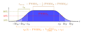
Figure 16.1: Emitted GAUSS and FLATTOP time profile with half-Gaussian edges and optional flat-top oscillations.

The rise and fall parameters correspond to \[ \mathrm{TRISE} = 1.6869\,\sigma_R, \qquad \mathrm{TFALL} = 1.6869\,\sigma_F, \] and the pulse FWHM is \[ \mathrm{TPULSEFWHM} = t_{\mathrm{flattop}} + \sqrt{2\ln 2}(\sigma_R + \sigma_F). \]

The total emission time depends on CUTOFFLONG: \[ t_E = \mathrm{TPULSEFWHM} + \frac{\mathrm{CUTOFFLONG} - \sqrt{2 \ln 2}}{1.6869} (\mathrm{TRISE} + \mathrm{TFALL}). \]

Correlations for GAUSS

The Gaussian generator also supports experimental correlations. They can be given either as a compact array R or through named coefficients such as:

• CORRX, CORRY, CORRZ
• R51, R52
• R61, R62

In the four-dimensional (x, p_x, z, p_z) subspace, the correlation matrix is \[ \sigma = \begin{bmatrix} 1 & c_x & R_{51} & R_{61} \\ c_x & 1 & R_{52} & R_{62} \\ R_{51} & R_{52} & 1 & c_t \\ R_{61} & R_{62} & c_t & 1 \end{bmatrix}. \]

The implementation constructs correlated samples from the Cholesky factorization of this matrix. This feature is experimental and only documented for Gaussian distributions.

16.7.3 FLATTOP

FLATTOP defines hard-edge distributions and is commonly used to model laser profiles in photoinjectors.

Injected FLATTOP

For injected beams, the distribution is a uniformly filled ellipse transversely and uniform in z.

Attribute	Meaning
SIGMAX, SIGMAY	Hard-edge widths.
SIGMAR	Radial hard-edge width; overrides SIGMAX and SIGMAY.
SIGMAZ	Hard-edge bunch length.

Emitted FLATTOP

For emitted beams, FLATTOP uses the same longitudinal pulse-shape parameters as the photoinjector-style GAUSS case.

Additional attributes include:

Attribute	Meaning
SIGMAX, SIGMAY, SIGMAR	Hard-edge transverse beam size.
SIGMAT, TPULSEFWHM, TRISE, TFALL	Time-profile parameters.
FTOSCAMPLITUDE, FTOSCPERIODS	Oscillations on the flat top.
LASERPROFFN, IMAGENAME, INTENSITYCUT	Laser-profile image input.
FLIPX, FLIPY, ROTATE90, ROTATE180, ROTATE270	Laser-image transforms.

Example:

Dist: DISTRIBUTION, TYPE = FLATTOP,
      SIGMAX = 0.001,
      SIGMAY = 0.002,
      TRISE = 0.5e-12,
      TFALL = 0.5e-12,
      TPULSEFWHM = 10.0e-12,
      CUTOFFLONG = 4.0,
      NBIN = 5,
      EMISSIONSTEPS = 100,
      EMISSIONMODEL = ASTRA,
      EKIN = 0.5,
      EMITTED = TRUE;

The legacy manual also describes a laser-image driven transverse sampling path through LASERPROFFN, but explicitly marks it as under development.

GUNGAUSSFLATTOPTH and ASTRAFLATTOPTH

These are legacy shorthands for emitted flat-top photoinjector distributions. Both correspond to FLATTOP-style emission. GUNGAUSSFLATTOPTH automatically enables EMITTED=TRUE and EMISSIONMODEL=ASTRA, while ASTRAFLATTOPTH follows the same idea with a slightly different legacy longitudinal profile generator.

16.7.4 BINOMIAL

BINOMIAL generates a family of distributions governed by one parameter m per axis. Changing m moves continuously from hollow-shell and flat-profile shapes toward Gaussian-like limits [1].

Figure 16.2: Representative transverse properties of binomial phase-space distributions.

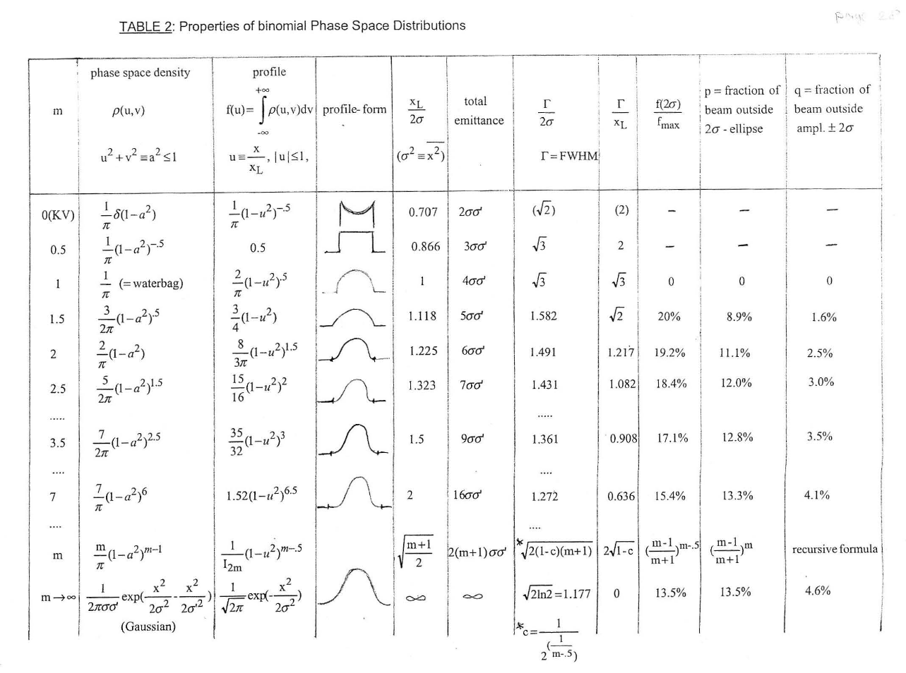
The key shape parameters are:

Attribute	Meaning
MX	Binomial parameter in x.
MY	Binomial parameter in y.
MT, MZ	Binomial parameter in the longitudinal direction. MZ is the same as MT.

The phase-space widths are still set through the usual SIGMAX, SIGMAPX, CORRX, and corresponding y and z/t variants.

For one plane, \[ \epsilon_x = \sigma_x \sigma_{x'} \cos\!\left(\arcsin(\sigma_{12})\right), \] with the corresponding Twiss relations \[ \beta_x = \frac{\sigma_x^2}{\epsilon_x}, \qquad \gamma_x = \frac{\sigma_{x'}^2}{\epsilon_x}, \qquad \alpha_x = -\sigma_{12}\sqrt{\beta_x \gamma_x}. \]

Example:

Dist: DISTRIBUTION, TYPE    = BINOMIAL,
      SIGMAX  = 2.15e-03,
      SIGMAPX = 1E-6,
      CORRX   = 0.0,
      MX      = 0.01,
      SIGMAY  = 0.50*23.e-03,
      SIGMAPY = 28.0,
      CORRY   = 0.5,
      MY      = 990.0,
      SIGMAT  = 1.0e-1,
      SIGMAPT = 11.96,
      CORRT   = -0.5,
      MT      = 2.0;

16.7.5 GAUSSMATCHED

GAUSSMATCHED constructs a matched Gaussian distribution, intended for cyclotron-style matched injection. The main control parameters are:

Attribute	Meaning
DENERGY	Energy step size for the closed-orbit finder.
EX, EY, ET	Projected normalized emittances.
NSTEPS, NSECTORS	Closed-orbit integration controls.
SECTOR	Match using one sector or the full ring.
ORDERMAPS	Order used in the field expansion.
RGUESS	Initial radius guess.
RESIDUUM	Convergence target.
MAXSTEPSCO, MAXSTEPSSI	Iteration limits for the closed-orbit and matching loops.

The legacy manual explicitly notes one limitation: trim-coil field maps are not included in this matched-distribution construction.

16.7.6 MULTIGAUSS

MULTIGAUSS models a train of Gaussian pulses. Transversely it uses a uniform elliptical profile, while longitudinally it generates NPEAKS equally spaced Gaussian peaks [2].

Key attributes are:

Attribute	Meaning
SIGMAX, SIGMAY, SIGMAR	Transverse size.
SIGMAZ, SIGMAT	RMS length of each Gaussian pulse.
SEPPEAKS	Peak-to-peak separation.
NPEAKS	Number of Gaussian pulses.
CUTOFFLONG	Longitudinal cutoff relative to the first and last pulse.
SIGMAPX, SIGMAPY, SIGMAPZ	Momentum spread for injected beams.
CUTOFFPX, CUTOFFPY, CUTOFFPZ	Momentum cutoffs for injected beams.

When emitted, the momentum is assigned by the selected emission model. When injected, the momentum components are sampled from normal distributions.

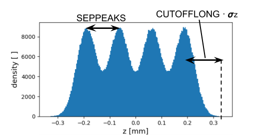
Figure 16.3: Example of an injected MULTIGAUSS bunch with several separated longitudinal peaks.

Example:

Dist: DISTRIBUTION, TYPE = MULTIGAUSS,
      SIGMAPX = 1e-2, SIGMAPY = 1e-2, SIGMAPZ = 1e-2,
      CUTOFFPX = 4.0, CUTOFFPY = 4.0, CUTOFFPZ = 4.0,
      SIGMAR = 340e-6,
      SIGMAZ = 90e-6 / 2.355,
      CUTOFFLONG = 4.0,
      SEPPEAKS = 126e-6,
      NPEAKS = 4,
      EMITTED = FALSE;

16.8 Emission Models

Emission models apply only to emitted distributions and determine how thermal energy and cathode physics are translated into initial particle momentum.

16.8.1 NONE

NONE is the default OPAL-T emission model. It adds a user-specified kinetic energy EKIN to the longitudinal momentum only.

Attribute	Default	Meaning
EKIN	1.0 eV	Thermal energy added during emission.

This model is useful for transversely cold emitted beams. If EKIN=0, emitted particles may fail to drift off the cathode cleanly.

16.8.2 ASTRA

ASTRA uses the same EKIN parameter but distributes the momentum three-dimensionally: \[ p_{\mathrm{total}} = \sqrt{\left(\frac{\mathrm{EKIN}}{mc^2}+1\right)^2 - 1}, \] \[ p_x = p_{\mathrm{total}}\sin(\theta)\cos(\phi),\quad p_y = p_{\mathrm{total}}\sin(\theta)\sin(\phi),\quad p_z = p_{\mathrm{total}}|\cos(\theta)|. \]

Here theta is random on [0, pi], and \[ \phi = 2 \arccos\!\left(\sqrt{x}\right), \] with x a uniform random number on [0, 1].

16.8.3 NONEQUIL

NONEQUIL is a more physical photoemission model for metal cathodes and materials such as CsTe [3], [4], [5].

Its additional parameters are:

Attribute	Default	Meaning
ELASER	4.86 eV	Drive-laser photon energy.
W	4.31 eV	Cathode work function.
FE	7.0 eV	Fermi energy.
CATHTEMP	300 K	Cathode temperature.

Example:

Dist: DISTRIBUTION, TYPE = GAUSS,
      SIGMAX = 0.001,
      SIGMAY = 0.002,
      TRISE = 1.0e-12,
      TFALL = 1.0e-12,
      TPULSEFWHM = 15.0e-12,
      CUTOFFLONG = 3.0,
      NBIN = 10,
      EMISSIONSTEPS = 100,
      EMISSIONMODEL = NONEQUIL,
      ELASER = 6.48,
      W = 4.1,
      FE = 7.0,
      CATHTEMP = 325,
      EMITTED = TRUE;

16.9 Distribution List

The RUN command can accept either a single distribution or a list:

RUN, METHOD = "PARALLEL-T",
     BEAM = beam_name,
     FIELDSOLVER = field_solver_name,
     DISTRIBUTION = DIST1;

or

RUN, METHOD = "PARALLEL-T",
     BEAM = beam_name,
     FIELDSOLVER = field_solver_name,
     DISTRIBUTION = {DIST1, DIST2, DIST3};

In a distribution list:

• the first entry is the master distribution
• all other distributions inherit its EMITTED or injected mode
• the total number of particles is still controlled by the BEAM command
• per-distribution particle counts are apportioned through WEIGHT

FROMFILE is the special case: its particle count comes from the file rather than from BEAM and WEIGHT.

[1]

W. Joho, “Representation of beam ellipses for transport calculations,” Paul Scherrer Institute, TM-11-14, 1980. Available: https://indico.psi.ch/event/3484/attachments/5948/7502/TM-11-14.pdf

[2]

J. G. Power and C. Jing, “Temporal laser pulse shaping for RF photocathode guns: The cheap and easy way using UV birefringent crystals,” in AIP conference proceedings, 2009, p. 689. doi: 10.1063/1.3080991.

[3]

K. Fl"ottmann, “Note on the thermal emittance of electrons emitted by cesium telluride photo cathodes,” Deutsches Elektronen-Synchrotron, DESY-TESLA-FEL-97-01, 1997.

[4]

J. E. Clendenin et al., “Reduction of thermal emittance of RF guns,” Nuclear Instruments and Methods in Physics Research Section A, vol. 455, p. 198, 2000, Available: https://www.sciencedirect.com/science/article/pii/S0168900200007312

[5]

D. H. Dowell and J. F. Schmerge, “Quantum efficiency and thermal emittance of metal photocathodes,” Physical Review Special Topics - Accelerators and Beams, vol. 12, p. 074201, 2009, doi: 10.1103/PhysRevSTAB.12.074201.