35 DB & DBA with Fringe Fields
35.1 Additional unpadded six-cell RING
The separate sandbox/map-3/ring/build_ring.py fixture assembles six unchanged 60-degree DBA cells using explicit 6D entrance poses. It retains \(\rho=2\) m, two 30-degree bends, two 1 m drifts and the 0.2 m quadrupole per cell, with HGAP=0.1, FINT=0.1 and the existing unmatched quadrupole seed. Its design circumference is
\[ C_{\mathrm{design}}=6\left(2\rho\frac{\pi}{6}+2(1\,\mathrm m)+0.2\,\mathrm m\right) =25.7663706143592\,\mathrm m. \]
No fringe padding is added. Thus this is different geometry from the historical separated-support cell studied below, not a reproduction of its matrix. The existing study inputs, results and provenance remain unchanged. Finite transverse apertures distinguish neighbouring ring sectors: horizontal half-width 0.5 m, vertical half-width 0.1 m. These are transverse domain choices, not longitudinal field cutoffs or changes to the native fringe formulas.
The generator checks nominal position/direction closure and contiguous body intervals. Its optional OPALX run uses MAXSTEPS=1 and --info 2, saving map-3-ring.out, geometry and provenance. The default DOP853, \(\Delta t=10^{-11}\) s, \(\epsilon_j=10^{-4}\) and one Richardson level are smoke-test settings, not a new optimum or convergence claim. See geometry, fringe support and ring return for the distinction between design closure and a tracked closed orbit.
35.1.1 Initial ring validation
The dop853-validation run completed with those settings and printed a finite \(6\times6\) return matrix. The unchanged quadrupole seed and launch are not matched to the unpadded ring:
| Quantity | Value |
|---|---|
| Design circumference | 25.7663706144 m |
| Reference return length | 25.3196055628 m |
| Return position mismatch | 0.601429057145 m |
| Relative momentum mismatch | 0.388948624674 |
| \(R_{16}\) | 6.346340692238 m |
| \(R_{26}\) | 1.343525845901 |
| Printed \(\lvert\det M-1\rvert\) | 0.36949810 |
| Printed \(\max_{ij}\lvert(M^TJM-J)_{ij}\rvert\) | 68.898765 |
These are return-map diagnostics, not an accuracy or symplecticity pass. The large matrix entries and mismatch require a closed-orbit/optics study before using this case as an optics regression oracle. The reported coordinates include noncanonical slopes, and the final momentum is not normal to the reused section; neither printed residual alone identifies the numerical integration error. No retuning, fringe renormalization or tolerance relaxation was applied. The executable SHA-256 was independently checked before and after the run: f1a53f9b26b42566c0ad367bf4125d22ba819c06c8e8be24c486dec2202e300e. The input, stdout and result provenance are in sandbox/map-3/ring/dop853-validation/. This smoke run validates completion and the separation of geometry from travelled length, not orbit closure.
35.2 Historical separated-support cell study
This first stage of sandbox/map-3 defines the analytic fields, not an exact transfer matrix or a matched achromat. It follows BendFieldModel.h, SBend::makeFieldInputs, OpalSBend::update and PlacementResolver on the 546-add-linear-transfer-matrix-to-each-elemen development branch. The initial field-definition stage contains no tracking. The subsequent three-case OPALX reproduction is reported below.
The coordinate \(s\) is distance along the nominal placed design line: straight entrance tangent, sector arc, straight exit tangent. It is not the path length of a numerically tracked reference particle. Field components use the local design-line basis \((x,y,s)\); \(B_s\) must not be confused with laboratory \(B_z\). For this horizontal, unrolled lattice, \(B_y\) is also the laboratory vertical field.
35.3 Layout with separated supports
Keep the map-2 body radius \(\rho=2\,\mathrm{m}\), angle \(\theta=\pi/6\), length \(L_b=\rho\theta=1.047197551197\,\mathrm{m}\), quadrupole length \(L_q=0.2\,\mathrm{m}\) and two field-free drifts of \(L_d=1\,\mathrm{m}\) each. The agreed fringe parameters are
\[ \mathrm{HGAP}=0.1\,\mathrm{m},\qquad \mathrm{FINT}=0.1,\qquad g=2\,\mathrm{HGAP}=0.2\,\mathrm{m},\qquad w=5g=1\,\mathrm{m}. \]
Here \(g\) is the full gap and \(w\) is the support extension on each side of a bend body. FINT is dimensionless and does not set this support width. For a body entrance at \(s_b\), the support is \([s_b-w,s_b+L_b+w)\). ELEMEDGE would specify \(s_b\), the geometrical body entrance, not the support entrance.
| Element | Support interval [m] | Nominal body interval [m] |
|---|---|---|
| B1 | 0.000000–3.047198 | 1.000000–2.047198 |
| D1 | 3.047198–4.047198 | same |
| QACH | 4.047198–4.247198 | same |
| D2 | 4.247198–5.247198 | same |
| B2 | 5.247198–8.294395 | 6.247198–7.294395 |
Thus \(L_{\mathrm{total}}=2L_b+4w+2L_d+L_q=8.294395102393\,\mathrm{m}\). Supports touch but do not overlap along this nominal line. D1/D2 contain no bend fringe. This is not yet a verification of the actual tracked orbit’s three-dimensional element membership or aperture clearance.
35.4 Source-matched Enge envelope
Let \(z=s-s_b\) be the local longitudinal coordinate relative to a bend body entrance. The pole-face function is
\[ F(d)=\frac{1}{1+\exp P(u)},\qquad u=\frac{d}{g},\qquad P(u)=\sum_{i=0}^{5}c_i u^i, \]
with \(d<0\) inside the face and
\[ (c_0,c_1,c_2,c_3,c_4,c_5)= (0.478959,1.911289,-1.185953,1.630554,-1.082657,0.318111). \]
The current code uses
\[ A(z)=\min\{F(-z),F(z-L_b)\}. \]
The smaller envelope selects the active face; a tie selects the entrance. The external support mask sets the field to zero outside \([-w,L_b+w)\). For \(g=0\), the profile is one with zero derivatives, and the support is simply \([0,L_b)\), giving the hard-edge limit. The exponential is saturated at \(P>80\) (\(F=0\)) and \(P<-80\) (\(F=1\)), with zero derivatives there.
Writing \(P_d=dP/dd\) and \(P_{dd}=d^2P/dd^2\), the unsaturated derivatives are
\[ F_d=-P_dF(1-F),\qquad F_{dd}=F(1-F)\left[(1-2F)P_d^2-P_{dd}\right]. \]
For the entrance face \(A'=-F_d(-z)\); for the exit \(A'=F_d(z-L_b)\). In either case \(A''\) is the active face’s \(F_{dd}\). Primes on \(A\) mean derivatives with respect to \(z\), in \(\mathrm{m}^{-1}\) and \(\mathrm{m}^{-2}\). The Python implementation uses the equivalent exponential expressions to retain small derivatives when the floating-point value of \(F\) rounds to one.
This is the development branch’s Enge model, not the older linear-ramp description. No effective-length rescaling is applied by OpalSBend::update.
35.5 Magnetic components and FINT
For the field normalization, \(p_0=0.2505104781131461\,\mathrm{GeV}/c\), \(q=-e\) and \(h=1/\rho=0.5\,\mathrm{m}^{-1}\). The physical dipole field is
\[ B_0=\frac{p_0}{q}h=-0.4178065048473403\,\mathrm{T}, \]
where \(p_0/q\) is evaluated in SI units. Numerically, for momentum supplied in \(\mathrm{GeV}/c\), the rigidity in tesla-metres is \(B\rho=10^9p_0/[(q/e)c]\), with \(c=299792458\,\mathrm{m/s}\).
The sector faces have zero pole-face rotation. Do not specify E1 or E2: those attributes are currently rejected. The FINT coefficient is
\[ \psi=h\,\mathrm{HGAP}\,\mathrm{FINT},\qquad k_y=h\tan\psi,\qquad S=|F(-w)-F(w)|,\qquad C=\frac{B_0}{h}\frac{k_y}{S}. \]
\(\psi\) is an angle in radians, \(k_y\) is in \(\mathrm{m}^{-1}\) and \(C\) is in tesla. For a pure dipole, the current source’s local field components are
\[ \begin{aligned} B_x &= \sigma C A'(z)y, &\sigma&=\begin{cases}+1&\text{entrance active},\\-1&\text{exit active},\end{cases}\\ B_y &= B_0\left[A(z)-\frac12 A''(z)y^2\right],\\ B_s &= B_0 A'(z)y. \end{aligned} \]
All fields are in tesla and offsets in metres. This reproduces the native near-axis field law; it does not assert an exact global vacuum-Maxwell solution. The active-face minimum is piecewise defined, and the external support is truncated. High-order integration cannot unconditionally assume global smoothness. For the selected dimensions the envelope reaches the full-field plateau before the active-face switch.
On the centreline \(x=y=0\), \(B_x=B_s=0\) and \(B_y=B_0A(z)\). Consequently FINT is invisible in the centreline field plot. The additional diagnostic samples a fixed \(x=0\), \(y=1\,\mathrm{mm}\) offset and isolates \(\Delta B_x=B_x(\mathrm{FINT}=0.1)-B_x(\mathrm{FINT}=0)\). Entrance and exit have the same sign of \(\Delta B_x\); \(B_s\) reverses sign. These are probes of the field, not tracked rays.
The central standalone quadrupole has \(B_x=Gy\), \(B_y=Gx\), \(B_s=0\). Retaining the old map-2 value \(K_1=-6.371966681365967\,\mathrm{m}^{-2}\) only as an unmatched seed gives \(G=-5.324498256290442\,\mathrm{T/m}\). This sign follows the current OpalQuadrupole/Multipole convention \(G=(10^9p_0/c)K_1\), which does not include SBEND’s division by reference charge. The quadrupole field therefore vanishes on its nominal centreline even though its gradient is nonzero.
35.6 Field integral and next validation
Adaptive numerical quadrature of the analytic profile gives, for either bend,
\[ \begin{aligned} L_{\mathrm{eff}}&=\int_{-w}^{L_b+w} A(z)\,dz =1.047200488015433\,\mathrm{m},\\ \int B_y\,ds&=B_0L_{\mathrm{eff}}=-0.4375271757721572\,\mathrm{T\,m}. \end{aligned} \]
The estimated quadrature error is \(7.0\times10^{-13}\,\mathrm{m}\); this is not a field-model accuracy bound. The default coefficients nearly balance the field lost inside and added outside: \(L_{\mathrm{eff}}-L_b\simeq2.94\,\mu\mathrm{m}\). The nominal-line curvature integral \(hL_{\mathrm{eff}}\) corresponds to \(30.00008413^{\circ}\), not a prediction of actual orbit deflection. A ray already bends in the incoming fringe, whereas the nominal line is still straight.
The source repository’s sandbox/map-3/dba/analytic_fields.py generates the centreline and off-axis figures, sampled component table, support/body intervals and a summary containing the source-file hashes. Python tests check support separation, field-free drifts, derivatives, field signs, symmetry, FINT isolation and the hard-edge limit; TestBendFieldModel checks the C++ profile helpers.
Matching the actual reference orbit and dispersion remains future work. The unmatched lattice can already be compared with the independent reference below. The old map-2 hard-edge oracle is not valid for these fringe fields and larger body separation. Subsequent studies save stdout with --info 2.
35.7 OPALX reproduction with archived best settings
sandbox/map-3/dba/map-3-dba.in implements the fields and layout above, retaining the unmatched quadrupole seed and unscaled dipole strengths. Exactly one case per map integrator was run sequentially. MAXSTEPS=1 limits production tracking; the design OrbitThreader still computes the complete requested map to \(s=8.294395102393196\,\mathrm{m}\).
For each method, select the lowest full-map error among all saved valid map-2 observations. The previous campaign was incomplete, so these are observed minima, not a complete-grid optimum or a guarantee for map-3. The RK4 setting in particular may benefit from cancellation in the hard-edge benchmark. Each listed starting \(\epsilon\) is applied to all six coordinates, in metres or dimensionless units as appropriate.
| Integrator | \(\Delta t\) [s] | \(\epsilon\) | Richardson levels | \(R_{16}\) [m] | \(R_{26}\) |
|---|---|---|---|---|---|
| Boris | 1e-13 | 1e-5 | 1 | -1.976821004850 | -0.247747632004 |
| RK4 | 3e-11 | 3e-5 | 0 | -1.976824228889 | -0.247749986316 |
| DOP853 | 1e-11 | 0.003 | 1 | -1.976825802611 | -0.247748090546 |
All three runs completed and visited B1, D1, QACH, D2 and B2, with no recorded support overlaps. Logged fields in D1/D2 are exactly zero. Evaluate the analytic field at each logged global reference position, including the sector/tangent chart and placed element frames: this agrees with the logged OPALX field within the eight-significant-digit text precision. A comparison at equal nominal \(s\) would conflate field differences with the reference orbit’s displacement. Samples ambiguous at a hard quadrupole face after text rounding are counted separately and excluded from this pointwise field check: 0 Boris, 44 RK4 and 44 DOP853 samples. This is not a verification of integration accuracy or of off-axis FINT gradients from the on-plane reference samples alone.
The finite support is traversed slightly earlier in actual path length than the nominal layout suggests. For Boris, B2 ends near \(s=8.288374822\,\mathrm{m}\); the combined map includes the remaining field-free interval up to ZSTOP. The last design-path log entry is a trial midpoint recorded before endpoint localization and must not be interpreted as the final map plane.
| Integrator | \(\lvert\det M-1\rvert\) | \(\max_{ij}\lvert(M^TJM-J)_{ij}\rvert\) | OrbitThreader wall time [s] |
|---|---|---|---|
| Boris | 7.7564677e-9 | 9.6620733e-9 | 41.60 |
| RK4 | 1.0262537e-6 | 1.0222106e-6 | 2.898 |
| DOP853 | 1.7433327e-7 | 5.6822864e-7 | 19.49 |
The unchanged \(10^{-6}\) diagnostic threshold passes for Boris and DOP853; RK4 is slightly above it in both diagnostics. Canonical-\(J\) caveats from the map chapter still apply. Timing comes from each retained timing.dat and includes reference threading, map construction and related output. These are single observations at different settings, not a matched-accuracy efficiency comparison.
The largest entrywise differences over all 36 matrix entries are \(4.0507220\times10^{-5}\) (Boris–RK4), \(9.8690230\times10^{-6}\) (Boris–DOP853), and \(3.8389460\times10^{-5}\) (RK4–DOP853). These are cross-method differences, not errors relative to an analytic map. The large nonzero dispersion reflects the unmatched lattice, not a residual that should be compared with the map-2 achromat’s zero dispersion.
The source-tree runner and validator retain each full matrix, input, stdout with --info 2, timing, field/support data, and source/selection hashes in sandbox/map-3/dba/opalx-best-settings. No production numerical algorithms or tolerances were changed for these three runs. No OPALX convergence sweep was started; the subsequent independent reference calculation is described below.
35.8 CERN analytic edge map and convention check
Analytic linear fringe maps are available. For example, Silke Van der Schueren’s CERN lecture, Dipole fringing fields, 17 September 2024, slides 23–29 derives the fringe integral and gives the thin-edge matrix. In the usual full-gap convention, with face rotation \(E\) and signed curvature \(h\),
\[ \begin{aligned} K&=\frac{1}{g}\int_{-\infty}^{\infty} \frac{B_y(s)[B_0-B_y(s)]}{B_0^2}\,ds,\qquad g=2\,\mathrm{HGAP},\\ \psi_{\mathrm{CAS}}&=h g K\frac{1+\sin^2 E}{\cos E},\\ k_x&=h\tan E,\qquad k_y=-h\tan(E-\psi_{\mathrm{CAS}}). \end{aligned} \]
The integral is over one fringe, not both ends of a finite magnet. Here \(K=\mathrm{FINT}\). The full-gap definition and the same correction are also explicit in Zhang and Loulergue, IPAC 2013, equations 1–4. The edge matrix in \((x,x',y,y',\zeta,\delta)\) is the identity except \(R_{21}=k_x\) and \(R_{43}=k_y\). This linear matrix has determinant one and preserves the canonical \(J\); a finite-order nonlinear truncation is a different question.
For the present zero-rotation faces,
\[ \psi_{\mathrm{CAS}}=0.010\,\mathrm{rad},\qquad k_{y,\mathrm{CAS}}=0.005000166673\,\mathrm{m}^{-1}. \]
Source discrepancy, not corrected in this study: the current BendFieldModel::edgeVerticalKickCoefficient uses \(h\,\mathrm{HGAP}\,\mathrm{FINT}\), giving \(\psi=0.005\,\mathrm{rad}\) and \(k_y=0.002500020834\,\mathrm{m}^{-1}\). OpalSBend doubles HGAP into the stored full gap, and SBend::makeFieldInputs passes half that stored gap to the helper; there is no compensating factor of two. The existing unit test follows the current half-gap expression. These numbers compare the explicit edge coefficient, not the total focusing through the distributed fringe.
Furthermore, the current Enge profile is fixed by its coefficients and gap; FINT changes an added off-axis field term, not the profile’s integral \(K\). Consequently the distributed model cannot simply be identified with the CERN thin-edge model by inserting the same two input values. Changing that physical model requires a separate decision and validation, not a numerical tolerance adjustment.
compare_reference.py evaluates the analytic thin-edge DBA by composing its two body bend maps, four edge maps, central quadrupole and drifts. It retains all body positions: the two outer drifts are \(w\), and each inner body-to-quad drift is \(w+L_d\). This uses the nominal design orbit and rigidity, not the slightly displaced tracked orbit. It gives \(R_{16}=-1.929713679677\,\mathrm{m}\) and \(R_{26}=-0.207853671267\). The differences below are OPALX minus this different physical approximation:
| Integrator | \(\Delta R_{16}\) [m] | \(\Delta R_{26}\) | Largest scaled entry difference |
|---|---|---|---|
| Boris | -0.04710732517 | -0.03989396074 | 0.3926250678 |
| RK4 | -0.04711054921 | -0.03989631505 | 0.3926456112 |
| DOP853 | -0.04711212293 | -0.03989441928 | 0.3926349368 |
These are not integration-error estimates. In particular, the zero-rotation FINT edge correction changes only the vertical block, so the substantial horizontal/dispersion differences cannot be attributed to that coefficient’s factor of two. Distributed bending and the reference orbit also differ.
35.9 Independent distributed-field map comparison
To isolate numerical map errors for the fields actually run, independently integrate their variational Lorentz equations. This is a numerically evaluated analytic-field reference, not a closed-form solution and not a replacement for the CERN analytic approximation above.
Use actual particle path length \(\ell\) in metres, \(\mathbf k=\mathbf u/u_0\), \(\kappa=\lVert\mathbf k\rVert\), \(\mathbf n=\mathbf k/\kappa\) and \(\tau=\beta_0ct\) in metres, where \(\mathbf u=\boldsymbol\beta\gamma\). With \(\alpha=(q/e)c/[(mc^2)_{\mathrm{eV}}u_0]\) in \((\mathrm{T\,m})^{-1}\),
\[ \begin{aligned} \frac{d\mathbf r}{d\ell}&=\mathbf n, & \frac{d\mathbf k}{d\ell}&=\alpha\,\mathbf n\times\mathbf B(\mathbf r),\\ \frac{d\tau}{d\ell}&=\beta_0\frac{\sqrt{\kappa^2+u_0^{-2}}}{\kappa}, & \frac{dT}{d\ell}&=\frac{\partial f}{\partial z}T. \end{aligned} \]
Here \(z=(\mathbf r,\mathbf k,\tau)\), \(f=dz/d\ell\), and the \(7\times6\) matrix \(T\) differentiates this state with respect to the six entrance map coordinates. The source provides analytic field derivatives on the planar reference, including vertical derivatives needed for FINT. No shadow-ray differencing or OPALX calls are used. At a hard quadrupole face with state-space normal \(\nu=(\mathbf n_{\mathrm{face}},0,0,0,0)\), account for perturbed crossing times with
\[ T^+=\left[I+\frac{(f^+-f^-)\nu^T}{\nu^Tf^-}\right]T^-. \]
This is the saltation sensitivity update. At the end, project onto the common reference-normal plane before encoding slopes, \(\zeta=-\beta_{\mathrm{ref}}c\,\Delta t\), and relative momentum. The endpoint is the reference’s requested path length \(\ell=8.294395102393196\,\mathrm{m}\), including its final field-free interval.
The distribution uses \(u_0=490.23677597553325\). With the current electron mass \(mc^2=0.00051099895\,\mathrm{GeV}\) its momentum is \(0.2505104777748827\,\mathrm{GeV}/c\), slightly different from the explicit field-normalization P0 above. The reference preserves both values as run.
Adaptive SciPy DOP853 refinement gives a maximum entry change of \(2.0233\times10^{-11}\) between the last two settings; an independent RK45 integration differs by \(1.7714\times10^{-11}\). This is a convergence check, not a rigorous absolute error bound. The selected reference uses relative tolerance \(3\times10^{-14}\), absolute tolerance \(3\times10^{-16}\) and maximum path step \(0.005\,\mathrm{m}\). Its determinant and canonical-\(J\) residuals are \(1.24\times10^{-12}\) and \(9.97\times10^{-13}\) respectively.
Full-matrix tests cover exact drift, quadrupole and uniform relativistic bend; additional tests check the analytic field/Lorentz Jacobians, off-axis hard-face crossing sensitivity against independently integrated rays, momentum normalization and the DOP853/RK45 comparison. The tolerances in these independent Python checks do not modify OPALX’s existing diagnostics.
The distributed-field reference gives \(R_{16}=-1.976820978591533\,\mathrm{m}\) and \(R_{26}=-0.247747623262620\). Define \(\Delta M=M_{\mathrm{OPALX}}-M_{\mathrm{ref}}\). For an unambiguous dimensionless whole-map comparison, scale \(x,y,\zeta\) by \(L_*=1\,\mathrm{m}\) and leave slopes and relative momentum dimensionless. This is a coordinate scale, not an element length. Numerically the scaled entries equal the stored SI entries here.
| Integrator | \(\Delta R_{16}\) [m] | \(\Delta R_{26}\) | Maximum scaled entry error | Entry |
|---|---|---|---|---|
| Boris | -2.62585e-8 | -8.74138e-9 | 9.64778e-8 | \(R_{12}\) |
| RK4 | -3.25030e-6 | -2.36305e-6 | 4.05225e-5 | \(R_{34}\) |
| DOP853 | -4.82402e-6 | -4.67283e-7 | 9.96550e-6 | \(R_{12}\) |
These include all map-construction effects, not only the integrator’s local truncation error. Boris is closest at these particular archived settings; this does not establish an integrator ranking at equal cost or after tuning.
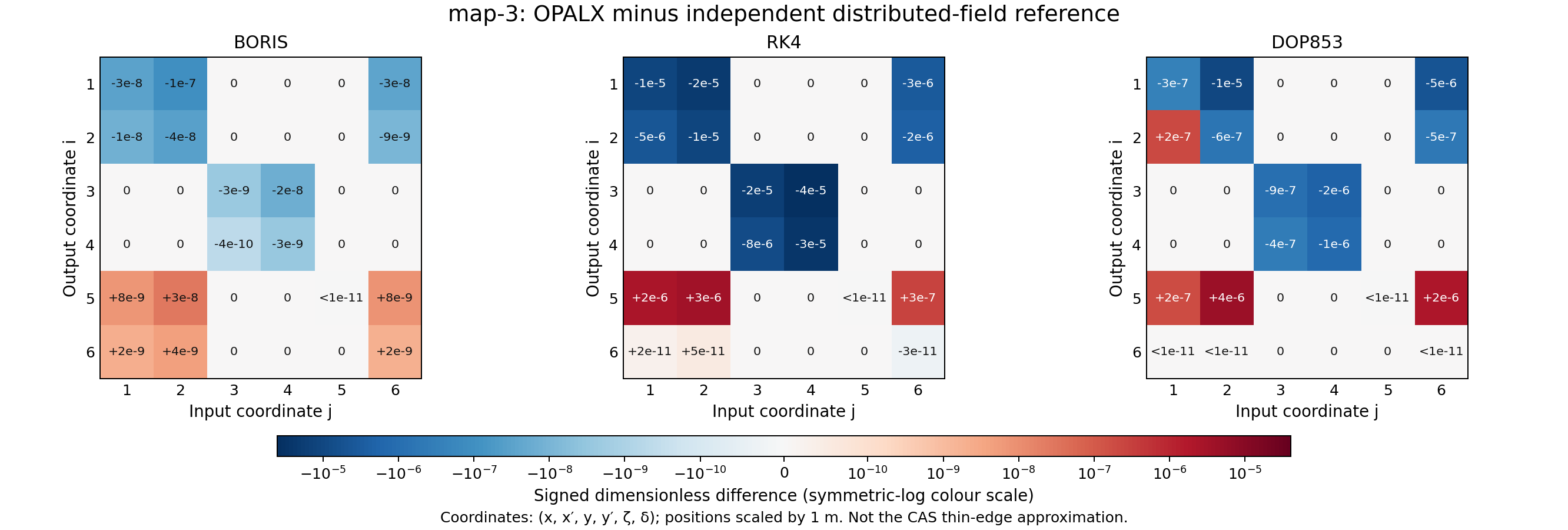
For the complete OPALX matrices, signed determinant errors calculated from the saved, text-rounded entries are approximately \(-7.76\times10^{-9}\) (Boris), \(-1.03\times10^{-6}\) (RK4), and \(-1.74\times10^{-7}\) (DOP853). OPALX stdout reports their absolute values before matrix text rounding; those more precise magnitudes remain in the earlier run table. Determinant one is necessary but not sufficient for symplecticity.
Reproduction scripts and tests are under sandbox/map-3/dba. The validated reference, refinements and source hashes are in variational-reference-validated/; map-comparison/ contains each full signed difference matrix, the separate CAS matrix, summary CSV, heatmap and provenance. The original three OPALX runs are unchanged. No new OPALX simulations or production-code changes were made for this comparison.