36 Beam-Beam
36.1 Scope and physical problem
Low-energy electron-positron pairs created near a gamma-gamma collider’s interaction point (IP) propagate through the electromagnetic fields of two counter-propagating primary electron bunches. OPALX calls the high-energy electron bunches primaries and the produced electrons and positrons witnesses. This chapter describes their transport, not pair production inside BEAMBEAM. CAIN supplies witness creation positions, momenta, and times. Photon and pair-production processes are a separate topic in Gamma-Gamma physics.
The implemented approximation tracks one physical primary. Its opposing partner is constructed by mirror symmetry about the IP, with the same charge and reversed longitudinal velocity. Witnesses sample these fields without depositing charge or feeding back on the primary. The benchmark additionally suppresses the primary’s collective kick with BBRIGID=TRUE.
The 12-witness benchmark verifies timed emission and transport in a prescribed symmetric primary model. Agreement with an independent like-for-like field model is sub-percent in the reported \(x\) and longitudinal trajectory norms. CAIN comparison gives approximately 9.5% in \(x\) and 3.0% longitudinally for the standard/fine cases, with larger relative discrepancies in weak components and some individual trajectories. CPU/A100 reproducibility is a third, separate result. These findings support a restricted initial implementation, not a claim of a fully converged, self-consistent two-beam collision model.
The BEAMBEAM element reference defines syntax, defaults, and supported combinations.
36.1.1 Geometry, source parameters, and units
For a placed element beginning at \(s_b\) with length \(L\), the IP is
\[ s_{\mathrm{IP}}=s_b+\frac{L}{2}. \]
The production geometry has \(s_b=0.01\) m, \(L=0.32\) m, and aperture radius \(0.15\) m, hence \(s_{\mathrm{IP}}=0.17\) m. The smaller Track-12 benchmark uses an 8 mm element with IP at 4 mm. Neither physical length sets the current numerical field-window length.
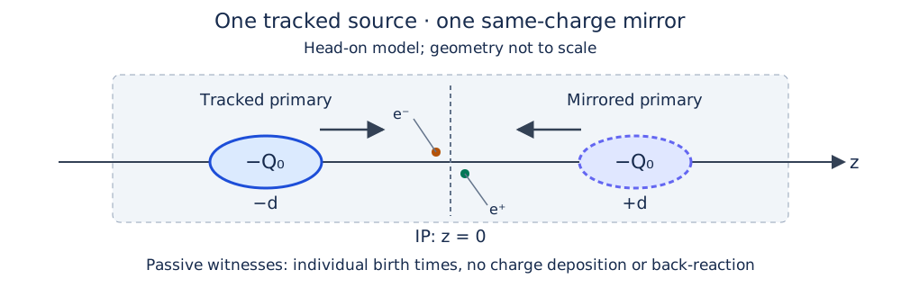
Let \(z=0\) denote the IP in the straight interaction frame. Primary centroids at \(-d\) and \(+d\) have centroid separation \(2d\). Distinguish this from the individual centroid-to-IP distance when specifying field probes or cutoffs.
| Quantity | Benchmark value |
|---|---|
| Primary kinetic energy \(K_0\) | 245 MeV |
| Electrons per primary \(N_e\) | \(1.25\times10^{10}\) |
| Charge per primary \(Q=-N_e e\) | \(-2.0027207925\times10^{-9}\) C |
| Laboratory transverse rms sizes \(\sigma_x=\sigma_y\) | \(1.944325075701\,\mu\mathrm m\) |
| Laboratory longitudinal rms size \(\sigma_z\) | \(0.6\) mm |
| Controlled source support | Component-wise \(\pm3\sigma_i\), renormalized |
| Track-12 witnesses | Six electrons and six positrons |
| Full CAIN population | 1,297 electrons and 1,297 positrons |
These are laboratory bunch dimensions. With \(\gamma_0=1+K_0/(m_ec^2)\), \(\beta_0=\sqrt{1-\gamma_0^{-2}}\), the reference momentum is \(p_0=\gamma_0\beta_0m_ec\). Input PC uses GeV/\(c\); particle-file momentum components use \(p/(m_ec)\). The positive input BCHARGE magnitude and electron species give negative physical source charge. Fields below use V/m and T; positions use metres.
36.2 Model and numerical field construction
36.2.1 Rigid source, quasi-static fields, and passive response
The frozen/rigid-source approximation is intentional. In the controlled benchmark, primary particles move with their prescribed initial momenta but do not receive the BeamBeam collective kick. Their charge still deposits on the mesh, and their changing positions still determine the solved field. BBRIGID therefore does not freeze a laboratory field forever, fix particle positions, or disable external fields. Suppressing collective forces alone also does not prevent ballistic expansion from an initially divergent source. The benchmark uses a nearly zero-divergence primary to approximate rigid translation; a finite-emittance production primary is a different model.
At a collective evaluation the source is treated electrostatically in its rest-frame approximation, then transformed back to laboratory electromagnetic fields. The resulting field is sampled for the tracker update and is not re-solved for every individual witness substep. This is not a full Maxwell evolution including radiation, retarded interaction between arbitrary bunches, or independent deformation of the opposing primary.
Only container 0 deposits charge for this interaction. Containers selected by WITNESS_CONTAINERS are passive: neither their self-fields nor their mutual forces enter the BeamBeam solve. Thus momentum/energy conservation for a closed system of both primaries and witnesses is not an expected property of the prescribed-source approximation. Numerical transport must instead be checked against the same specified fields.
36.2.2 Poisson solve and Lorentz transformation
For source velocity \(\mathbf v_s=c\boldsymbol\beta_s\) along \(z\), the event relative to its translating centroid is
\[ x'=x-x_c(t),\qquad y'=y-y_c(t),\qquad z'=\gamma_s[z-z_c(t)]. \]
The corresponding rms widths are \(\sigma_x'=\sigma_x\), \(\sigma_y'=\sigma_y\), and \(\sigma_z'=\gamma_s\sigma_z\). OPALX deposits the primary charge, solves the open-boundary rest-frame problem
\[ \nabla'^2\phi'=-\frac{\rho'}{\epsilon_0},\qquad \mathbf E'=-\nabla'\phi',\qquad \mathbf B'=0, \]
and forms laboratory fields. For a longitudinal boost,
\[ E_x=\gamma_s E_x',\qquad E_y=\gamma_s E_y',\qquad E_z=E_z', \qquad \mathbf B=\frac{\mathbf v_s\times\mathbf E}{c^2}. \]
The general vector electric-field conversion used by the composer is
\[ \mathbf E=\gamma_s\mathbf E'-(\gamma_s-1) (\mathbf E'\cdot\widehat{\mathbf v}_s)\widehat{\mathbf v}_s. \]
The benchmark uses one velocity bin and the integrated open Green function; the longitudinal mesh spacing is stretched by \(\gamma_s\) for the rest-frame solve. See Field Solver physics for the underlying PIC discretization.
36.2.3 Mirrored primary and one-solve composition
In the source-aligned coordinates, reflection maps
\[ \mathcal M(x,y,z)=(x,y,2z_{\mathrm{IP}}-z). \]
For a same-sign mirrored source,
\[ \rho_v(\mathbf r)=\rho_p(\mathcal M\mathbf r),\qquad \mathbf E'_v(\mathbf r) =\operatorname{diag}(1,1,-1)\mathbf E'_p(\mathcal M\mathbf r). \]
The copied mean momentum has its longitudinal component reversed; the same Lorentz conversion is then applied to the copied field. This is not an opposite-sign conducting-plane image charge. In the straight, head-on case, \(\mathbf v_v=-\mathbf v_p\) and
\[ \mathbf E_{\mathrm{tot}}=\mathbf E_p+\mathbf E_v,\qquad \mathbf B_{\mathrm{tot}}=\mathbf B_p+\mathbf B_v. \]
At exact overlap of identical symmetric primaries, the electric field doubles and the magnetic fields cancel. These are important sign and symmetry checks.
Because reflection and superposition are linear, the symmetric-domain implementation reuses one physical-source Poisson solve, reflects its field, and accumulates the two laboratory contributions. The common one-bin, no-cathode case therefore needs one backend solve per collective evaluation; an entry diagnostic can require an additional primary-only solve. Distributed reflection exchanges the required mesh regions, rather than assuming a slab decomposition. Field arrays remain in their configured Kokkos memory space. Multi-GPU distributed reflection requires a compatible GPU-aware MPI setup.
36.2.4 Witness equation of motion and frame mapping
For \(\mathbf P=\mathbf p/(m_ec)=\gamma\boldsymbol\beta\) and witness charge \(q=\pm e\), the continuous equations represented by the particle pusher are
\[ \frac{d\mathbf x}{dt}= c\frac{\mathbf P}{\sqrt{1+|\mathbf P|^2}},\qquad \frac{d\mathbf P}{dt}=\frac{q}{m_ec} \left[ \mathbf E_{\mathrm{tot}}+ c\frac{\mathbf P}{\sqrt{1+|\mathbf P|^2}}\times\mathbf B_{\mathrm{tot}} \right]. \]
Particle coordinates are stored relative to each container’s reference. Before interpolation they must be expressed in the primary source frame. For the straight longitudinal case,
\[ z_{\mathrm{source}}=z_{\mathrm{witness}}+ (s_{\mathrm{witness}}-s_{\mathrm{source}}). \]
The implementation also applies the reference-frame rotations/translations, gathers the distributed fields, and returns the sampled vectors to the witness tracking frame. All MPI ranks participate for a globally nonempty witness container, even when a rank owns no local witnesses. These details are essential for low-energy witnesses with reference motion very different from the high-energy primary.
36.3 Interaction window and mesh policy
The current numerical longitudinal window has fixed length \(L_f=20\) mm and boundaries \(s_\pm=s_{\mathrm{IP}}\pm L_f/2\). It is independent of physical aperture and element length. Let \(s_{\mathrm{tail}}\) be the minimum primary longitudinal coordinate.
| State | Transition and collective behaviour |
|---|---|
| Inactive | For known ELEMEDGE geometry, ordinary self-field solving is suppressed. Activate once \(s_{\mathrm{tail}}\ge s_-+L_f/(2N_z)\), including the implemented half-cell entry margin. |
| Active | Solve the primary field; include its mirror only when positive COPY_TIME has been reached; gather to configured witnesses. |
| Completed | Enter when \(s_{\mathrm{tail}}>s_+\). Restore the saved mesh configuration and stop BeamBeam solving/gathering. Ordinary self fields remain suppressed. Particles continue tracking; completion does not retire/delete the primary. |
A primary first encountered entirely downstream also becomes Completed. The policy is single-pass: a completed interaction is not reactivated. For absolute-pose placement, geometry discovery depends on the reference-orbit map; ELEMEDGE is the controlled straight-benchmark placement.
Transverse bounds include the source and configured witness populations, are padded using BBOXINCR, and never shrink during an active interaction. A second constraint limits excessive cell anisotropy in the source rest frame. With \(A_{\max}=1.5\times10^5\) and \(\Delta z'= \gamma_s L_f/(N_z-1)\), the minimum transverse span is
\[ W_{x,\min}=\frac{\Delta z'(N_x-1)}{A_{\max}},\qquad W_{y,\min}=\frac{\Delta z'(N_y-1)}{A_{\max}}. \]
This floor prevents extreme cell shapes encountered with the integrated Green function; it is not a physical accuracy criterion. More transverse mesh points can also enlarge the minimum permitted domain. Refinement must therefore record actual bounds and cell sizes, not only \((N_x,N_y,N_z)\).
The \(0.15\) m production aperture and \(1.944\,\mu\)m primary rms size remain widely separated scales. A coarse \(16^3\) production mesh is useful for a lifecycle/coverage check, not a converged prediction of kicks or pair losses. Dynamic transverse coverage does not guarantee longitudinal containment of all witnesses. Open particle boundaries must not be replaced by periodic wrapping to keep witnesses artificially inside the field domain.
36.4 CAIN input and exact birth timing
36.4.1 Full population
The CAIN fort98.txt table contains 1,297 electron-positron pairs. Paired particles have the same creation position and time, but different momenta. Creation times span \(-4.137532\) to \(+3.237053\) ps relative to the CAIN clock, with standard deviation \(1.037166\) ps. The mean kinetic energy is approximately 313.60 keV for each species; roughly half travel in each longitudinal direction. They are not a narrow paraxial witness beam.
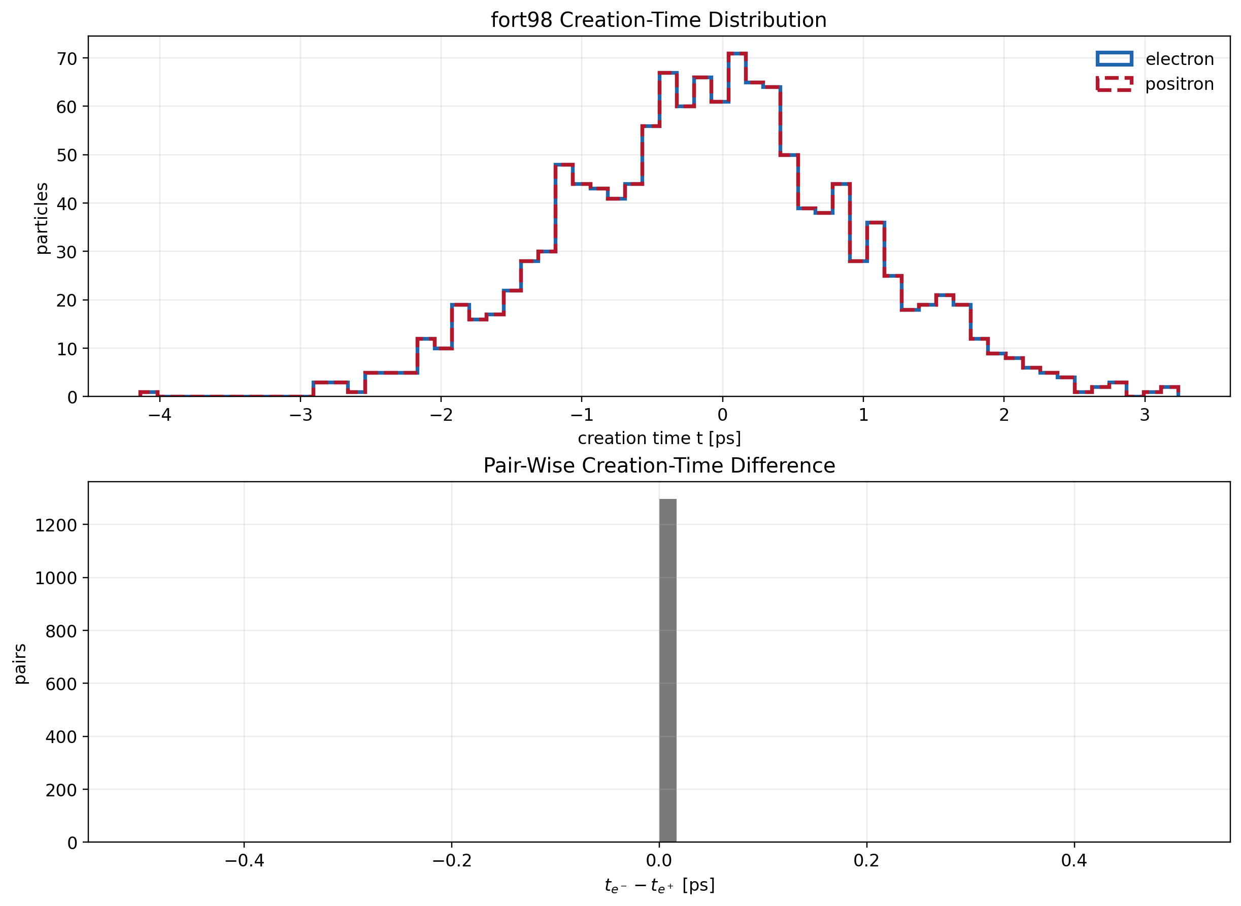
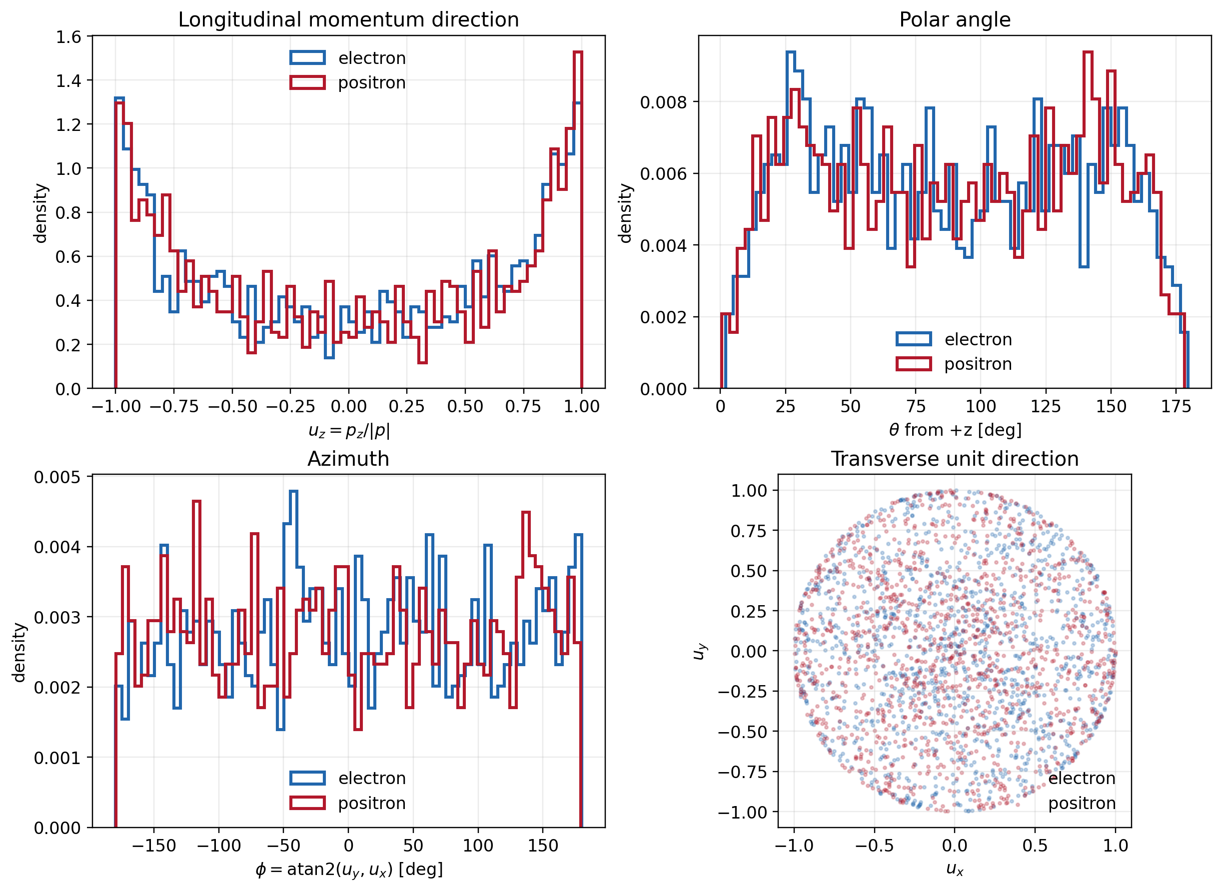
Convert CAIN \(ct\) in metres to time using \(t=ct/c\), and momentum in eV/\(c\) to \(\mathbf P\) by dividing by \(m_ec^2\) expressed in eV. Preserve species, identity, row pairing, and the creation clock. Emission-source offsets position the records at the OPALX IP and align their clock with primary overlap. EMITTEDFROMFILE carries x y z px py pz birth_time data after its count and column header; use separate distribution objects for the two species.
36.4.2 Controlled 12-witness comparison
The artificial reference contains six electrons and six positrons born at
\[ ct_b=(-0.9000,-0.5994,-0.3006,0,0.3006,0.5994)\ \mathrm{mm}. \]
CAIN samples every \(\Delta(ct)=1.8\,\mu\)m, so \(\Delta t=6.004153713566736\) fs, through \(ct=1.8\) mm. The OPALX preparation aligns these events to the same clock and includes an initial empty step to establish the fields before the first witness birth. The reference uses 1,501 steps and 13,012 comparison samples across all witnesses. These are 13,000 post-birth samples plus 12 initial birth states, not 13,012 samples per particle.
For a witness born within a step ending at \(t_{n+1}\), only
\[ \Delta t_i=t_{n+1}-t_{b,i} \]
is integrated. Exact boundary births and this fractional interval must be handled consistently. Comparisons align identity and physical time; they must not substitute row number for particle identity or silently interpolate over missing output. In the October reproduction, eight birth states were stored in H5 and four were reconstructed from the known input; all 13,000 post-birth records were measured.
36.5 Independent manufactured solution
For unchanging anisotropic Gaussian primaries in uniform motion, an independent evaluator uses the ellipsoidal Coulomb integral [1]. In a source rest frame, for displacement \(\mathbf r'\) from its centroid,
\[ E_i'(\mathbf r')= \frac{Q r_i'}{4\pi\epsilon_0\sqrt{2\pi}} \int_0^\infty \frac{\exp\left[-\frac12\sum_j r_j'^2/(\sigma_j'^2+u)\right]} {(\sigma_i'^2+u)\sqrt{\prod_j(\sigma_j'^2+u)}}\,du . \]
Here \(u\) has units of length squared and \(Q\) includes the charge sign. Logarithmic quadrature resolves the very large rest-frame aspect ratio. Each primary is evaluated in its own rest frame, Lorentz-transformed, and superposed in the laboratory frame. This evaluator does not call OPALX’s Poisson solver.
The untruncated expression alone is not a like-for-like oracle for a truncated particle input. The controlled comparisons instead integrate the component-wise three-sigma-truncated, renormalized density,
\[ \rho'_{\mathrm{tr}}(\mathbf r')= \frac{\rho'_G(\mathbf r')}{[\operatorname{erf}(3/\sqrt2)]^3} \prod_{j=x,y,z}\mathbf1_{\{|r_j'|\le3\sigma_j'\}}. \]
This is a rectangular component-wise cutoff, not a spherical radial cutoff. The independent witness integration uses both primaries, the exact birth events, and a maximum internal substep of 1 fs.
A retained physical-plus-mirrored field comparison with 20,301 probes at a centroid separation of \(3\sigma_z\) gives:
| Observable | Value |
|---|---|
| Maximum OPALX \(|\mathbf E|\) | \(5.545751\times10^9\) V/m |
| Maximum manufactured \(|\mathbf E|\) | \(5.553866\times10^9\) V/m |
| Relative \(L_2\) error of \(\mathbf E\) | 1.1098% |
| Relative \(L_2\) error of \(\mathbf B\) | 1.1098% |
| Median field-magnitude ratio | 0.997923 |
| Median direction cosine | 0.999970 |
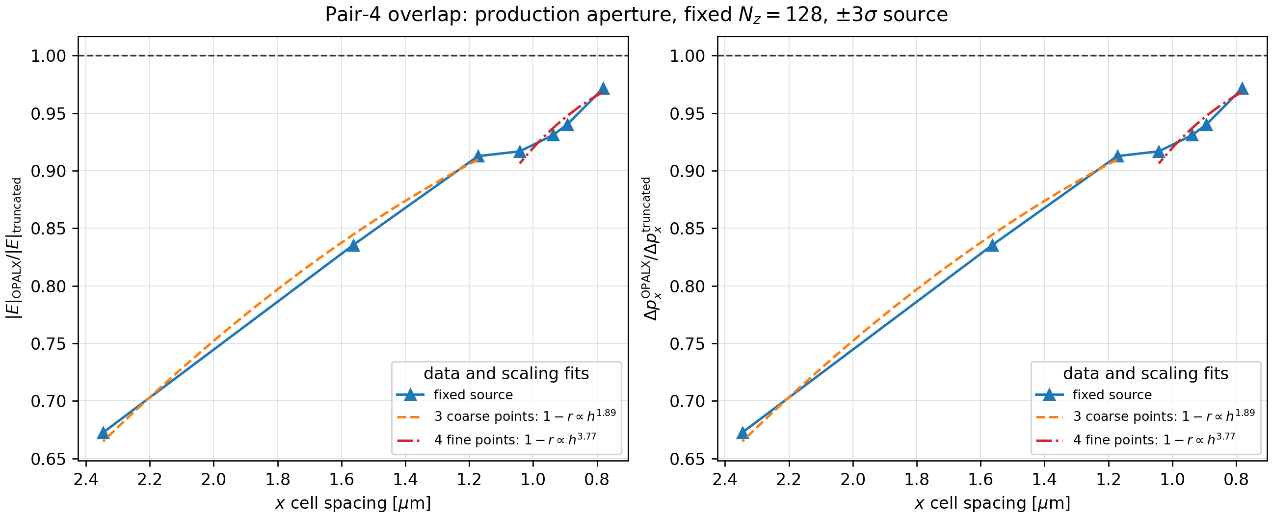
The first-kick scan holds the historical transverse box at \(2.4\) mm by \(0.24\) mm with \(N_z=128\). It shows a refinement trend approaching second order, with direction cosine at least 0.999993. Refining \(x\) while coarsening \(y\) need not improve the result; this historical fixed-box scan must not be conflated with current envelope-dependent domain sizing.
36.6 Results and their interpretation
36.6.1 Error measures
For matched samples \(a_k\) from OPALX and \(r_k\) from the stated reference,
\[ \epsilon_{L_2}(a,r)= \frac{\sqrt{\sum_k(a_k-r_k)^2}}{\sqrt{\sum_k r_k^2}}, \qquad \operatorname{RMSE}(a,r)= \sqrt{\frac1N\sum_k(a_k-r_k)^2}. \]
Tables report \(100\epsilon_{L_2}\) as percent. The longitudinal comparison coordinate \(s\) is aligned to the interaction-point convention of the reference. It is not an uncorrected container-local coordinate. A relative metric becomes undefined for an exactly zero reference norm and can be large for a small reference signal; report absolute errors as well. Overall norms also weight larger-amplitude trajectories more strongly than smaller ones.
36.6.2 Fine historical benchmark reported in the note
The retained fine run used 400,000 primary macroparticles, a \(4096\times256\times128\) mesh, four A100s, and the full 1,501-step clock. Its 13,012-sample comparisons are:
| Reference | \(x\) relative \(L_2\) | \(x\) RMSE (\(\mu\mathrm{m}\)) | \(s\) relative \(L_2\) | \(s\) RMSE (\(\mu\mathrm{m}\)) |
|---|---|---|---|---|
| Truncated manufactured model | 0.6004% | 1.996 | 0.0971% | 0.807 |
| CAIN | 9.5453% | 30.648 | 2.9774% | 24.477 |
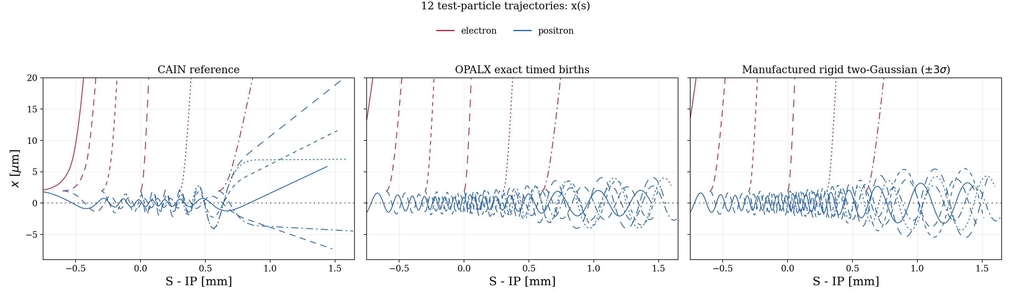
The twelve first-\(x\)-kick ratios to the truncated manufactured reference lie between 0.92947 and 0.97490, with mean 0.94860. The largest charge-conjugate kick residual is \(7.57\times10^{-10}\). These checks support species/sign, timing, and gather consistency; they do not independently establish equality of the CAIN and OPALX physical models.
This is a retained historical result, not a new run of the current release candidate. Its analyzer handled legacy particle-layout/identity conventions; the retained metadata records a periodic layout and multiple raw IDs per physical witness, although it reports no transverse wraps. The later open-boundary reproduction below is a distinct benchmark with stable IDs. The original note’s optimized one-solve comparison reported a 1.992-fold trajectory speedup, position changes below \(0.022\,\mu\)m and relative momentum changes below \(4\times10^{-6}\) versus its two-solve predecessor. That timing is campaign-specific, not a general performance guarantee.
36.6.3 October open-boundary reproduction
The standard A100 reproduction used 400,000 deterministic primaries, \(256\times256\times128\) cells, BBRIGID=TRUE, one velocity bin, GREENSF=INTEGRATED, and open particle boundaries. It completed all 1,501 steps and retained all twelve witness identities. No periodic unwrapping or time interpolation was needed.
| Reference | \(x\) relative \(L_2\) | \(x\) RMSE (\(\mu\mathrm{m}\)) | \(s\) relative \(L_2\) | \(s\) RMSE (\(\mu\mathrm{m}\)) |
|---|---|---|---|---|
| Truncated manufactured model | 0.8538% | 2.838 | 0.1173% | 0.975 |
| CAIN | 9.4828% | 30.447 | 2.9673% | 24.395 |
The aggregate \(x/s\) agreement is stable between these campaigns, but it does not describe every component or species. For the standard case:
| CAIN comparison | Relative \(L_2\) | RMSE (\(\mu\mathrm{m}\)) |
|---|---|---|
| All witnesses, \(y\) | 96.18% | 14.764 |
| Positrons only, \(x\) | 107.90% | 5.766 |
| Positrons only, \(s\) | 0.1019% | 0.881 |
The weak-component discrepancies are real limitations, not values to hide behind the aggregate norms. The rigid analytic model has zero reference \(y\) in this benchmark, so its relative \(y\) error is undefined; the OPALX \(y\) RMSE against that model is \(1.737\,\mu\)m.
CAIN uses a different collective-field treatment. Source emittance, truncation, force conventions, and the exact original input deck also need alignment before assigning the residual to a specific cause. The observed discrepancy is consistent with a model-comparison problem, but the study has not isolated its cause. Do not tune OPALX tolerances to force agreement with CAIN.
36.6.4 CPU/A100 reproducibility
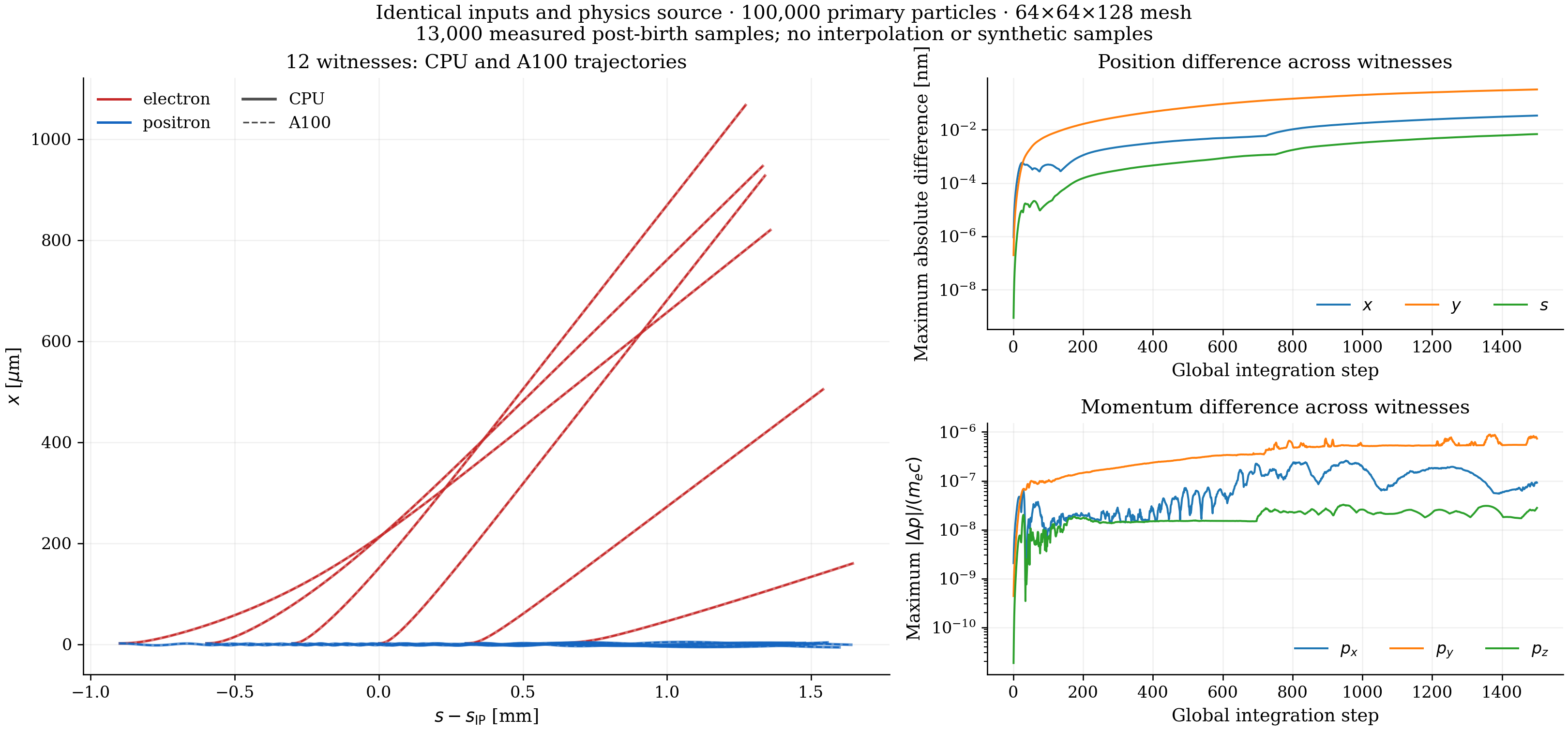
The architecture comparison uses identical 100,000-primary inputs and \(64\times64\times128\) cells on the local CPU and an A100. It is not a comparison of the small CPU mesh with the fine historical GPU mesh. Over 13,000 measured post-birth samples:
| Component | Maximum absolute CPU/A100 difference | Relative \(L_2\) |
|---|---|---|
| \(x\) | 0.03425 nm | \(2.6414\times10^{-8}\) |
| \(y\) | 0.32758 nm | \(1.1660\times10^{-5}\) |
| \(s\) | 0.00691 nm | \(1.7136\times10^{-9}\) |
| \(P_x\) | \(2.5921\times10^{-7}\) | \(8.4336\times10^{-8}\) |
| \(P_y\) | \(8.8306\times10^{-7}\) | \(1.8055\times10^{-5}\) |
| \(P_z\) | \(3.2528\times10^{-8}\) | \(5.6290\times10^{-9}\) |
Momentum differences are in \(p/(m_ec)\). The largest individual-witness/component relative \(L_2\) is 0.0491%, for an electron’s weak \(P_y\) component. The CPU and A100 CAIN \(x/s\) errors both remain approximately 8.2071%/3.0052% for this smaller setup. Excellent architecture agreement demonstrates reproducibility of the specified model, not agreement with a different model.
36.7 Supported scope and further validation
The supported initial scope is a straight, symmetric, single-pass interaction, with one physical primary, a mirrored partner, and configured passive witnesses. Multiple elements and repeated RING/TURNS passages are rejected. The controlled validation uses no cathode, one velocity bin, and the rigid primary approximation. It does not establish arbitrary crossing-angle, unequal-primary, radiation, witness back-reaction, or full-production loss accuracy.
The historical note proposed a centroid cutoff \(d=10\sigma_z=6\) mm: approximately \(\pm20\) ps around primary overlap at 245 MeV. This is not the implemented activation rule and is not an available element parameter. The current fixed 20 mm window is governed by the primary tail as described above. A Gaussian density is small at ten rms widths, but its electromagnetic field remains long-ranged; a physical cutoff needs a convergence study of the accumulated momentum kick.
Before interpreting 1,297-pair production losses, vary the timestep, actual field-domain bounds, mesh spacing, source macroparticle count, source truncation, and interaction cutoff. Check final momenta and positions, maximum transverse kick, aperture-loss counts/locations, and coverage for the complete witness population. Compact source meshes with controlled far-field evaluation or nested meshes are possible future methods, not current capabilities.
The large-cylinder staged production input still uses common-time FROMFILE injection. Do not confuse it with the separately validated individually timed full-population input. Align the production birth clock before interpreting that case as a complete timed CAIN comparison.
The full fine-grid CAIN comparison is extended validation, not a 20-30 second CI test. Short gtest/text-output regressions should protect field signs, source-only deposition, passive kicks, exact birth timing, rigid-source response, single-interaction guards, MPI ownership, and window transitions. This does not require new Python or HDF5 dependencies in the short regression suite.
36.8 Reproduction and evidence
The four studies are available together as a downloadable input-and-script bundle. Use the Download raw file button on the linked page to save the archive. The bundle preserves the shared launchers and cross-experiment analytic helpers; it contains no generated results, plots, OPALX executable, or Python environment.
The study workspace in the OPALX checkout is organized as:
| Directory | Purpose |
|---|---|
sandbox/experiment-1 |
Independent anisotropic fields and OPALX field comparisons |
sandbox/experiment-2 |
Exact-timed Track-12 CAIN/analytic comparisons |
sandbox/experiment-3 |
Full-population input conversion and exact emission checks |
sandbox/experiment-4 |
Production geometry, lifecycle, and cylinder diagnostics |
Each contains inputs/, scripts/, results/, and run.sh. sandbox/Experiments.md is the operational index. New runs record inputs, source/executable hashes, commands, and results. Default local launchers use coarse workflow profiles, not the fine benchmark settings above. Experiment 4 defaults to a primary-only lifecycle smoke; it does not track witnesses unless a full case is selected. The common --merlin6 launcher option is not yet implemented.
Extract the archive at the root of an OPALX Git checkout, retaining its sandbox/ directory structure. Check for existing experiment files first to avoid overwriting local work. The archive includes sandbox/Experiments.md and sandbox/DOWNLOAD.md with prerequisites and run instructions. Set OPALX_PYTHON to a Python interpreter with NumPy, SciPy, pandas, Matplotlib, and h5py installed, and select your built executable with --opalx:
tar -xzf /path/to/2026-10-06-beam-beam-experiments.tar.gz
export OPALX_PYTHON=/path/to/python
sandbox/experiment-1/run.sh --opalx /path/to/opalx --smoke
sandbox/experiment-2/run.sh --opalx /path/to/opalx --smoke
sandbox/experiment-3/run.sh --opalx /path/to/opalx
sandbox/experiment-4/run.sh --opalx /path/to/opalx
These are scientific study dependencies, not new requirements for the short regression suite. Results and analysis are generated under each experiment’s results/ directory. Historical analyses that require omitted output files must first regenerate or separately obtain those files.
The fine historical table, October standard table and CPU/A100 residuals come from archived comparison results. The matching preparation manifests and analyzer outputs recorded their settings and source truncation. The October campaign validated a source snapshot including the device field-clear fix; its executable/content fingerprints, not a bare branch name, identify the tested state. These historical result products are not included in the downloadable source bundle.
For reproducibility retain the exact particle-input hashes, source and executable fingerprints, field domain, mesh, timestep, truncation, MPI decomposition when comparing architectures, and complete identity/time-aligned output. Some obsolete raw field dumps and primary snapshots have been deleted to save space; their figures and comparison summaries remain. Regenerate missing raw diagnostics before claiming a fresh comparison.