9 γ-γ Physics
This note collects the physics model and benchmarks of the laser and photon functionality in OPALX.
9.1 Full Workflow
The top-level driver generate-gamma-gamma-results.sh regenerates the full published gamma-gamma benchmark state. It builds the required OPALX benchmark targets, runs the inverse-Compton and Breit-Wheeler physics tests, calls the shared CAIN helper scripts in ~/git/cain, and rerenders the physics notes.
Use it when you want to refresh all benchmark figures and note pages in one pass:
cd ~/git/OPALX-project.github.io/gamma-gamma
./generate-gamma-gamma-results.sh --opalx-build ~/git/opalx-laser/build_openmp
The narrower CAIN-side helpers remain useful when only one of the two physics notes needs to be regenerated.
9.2 Linear Compton Benchmark
9.2.1 Scope
This note documents the current OPALX validation path for linear inverse Compton scattering in the weak-field regime. The immediate goal is not yet a full tracking implementation, but a CAIN-validated benchmark path for the process
\[e^- + \gamma_L \rightarrow e^- + \gamma .\]
The benchmark follows the same staged strategy as the Breit-Wheeler note:
start from a fixed-geometry, unpolarized, linear process,
validate deterministic and sampled spectra against CAIN,
then extend to broader beam models without enabling tracked interaction yet.
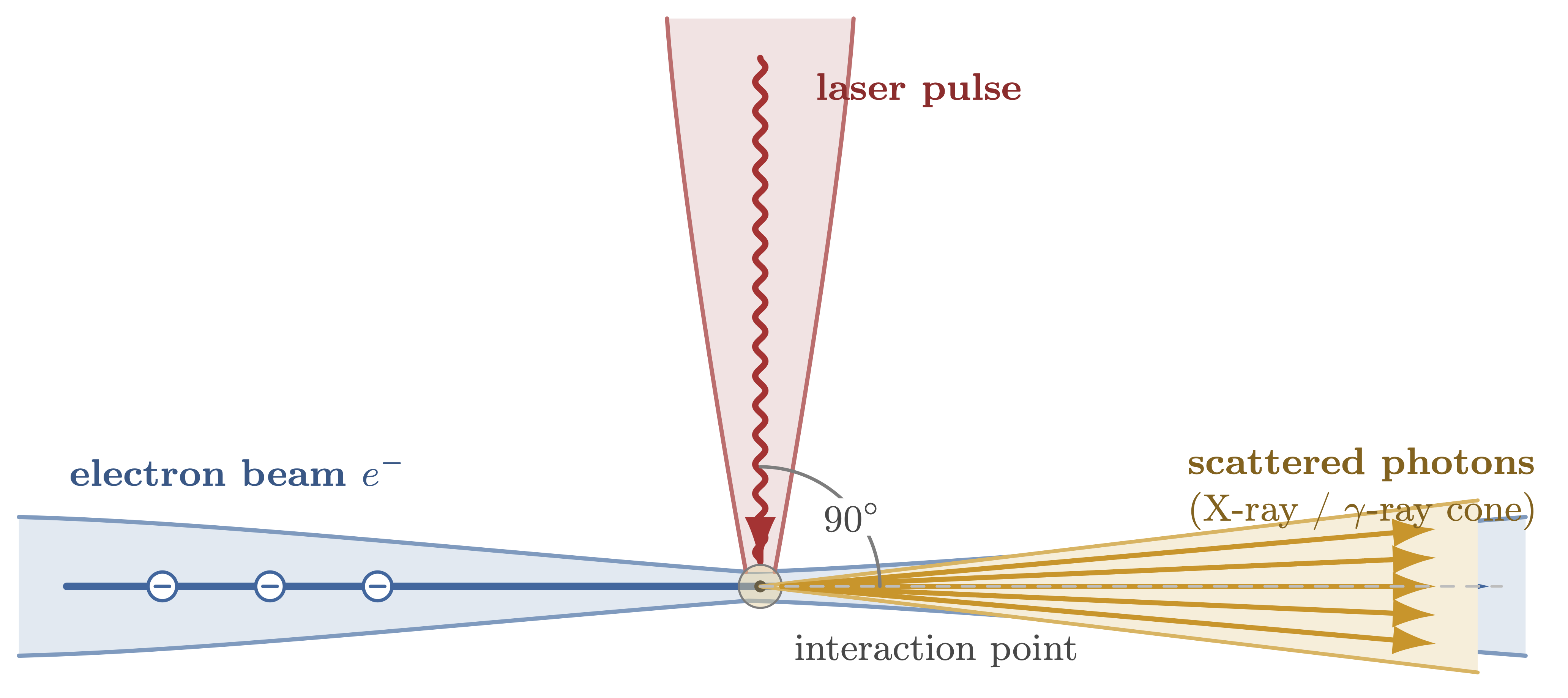
The baseline geometry used here is a \(90^\circ\) crossing between a 1 GeV electron beam along \(\hat z\) and a laser photon beam along \(\hat x\) with wavelength 1030 nm.
9.2.2 Physics Models
Basic Kinematics
For a laser wavelength \(\lambda_L\), the photon energy is
\[ \omega_L = \frac{2 \pi \hbar c}{\lambda_L} . \tag{9.1}\]
For an electron with total energy \(E_e\) and momentum magnitude \(p_e = \sqrt{E_e^2 - m_e^2}\), the exact forward-scattered photon energy in the 90 degree benchmark geometry is
\[ \omega_\gamma' = \frac{E_e \, \omega_L} {\omega_L + \frac{m_e^2}{E_e + p_e}} . \tag{9.2}\]
The current OPALX helper uses this numerically stable form directly in the unit benchmark.
Rest-Frame Model
The exact linear Compton kernel is evaluated in the electron rest frame. Let \(\omega_1\) be the incoming photon energy there and let \(\Theta^*\) be the photon scattering angle. The scattered photon energy is
\[ \omega_2(\Theta^*) = \frac{\omega_1} {1 + (\omega_1/m_e)(1 - \cos \Theta^*)} . \tag{9.3}\]
The unpolarized Klein-Nishina differential cross section is
\[ \frac{d\sigma}{d\Omega^*} = \frac{r_e^2}{2} \left(\frac{\omega_2}{\omega_1}\right)^2 \left( \frac{\omega_1}{\omega_2} + \frac{\omega_2}{\omega_1} - \sin^2 \Theta^* \right) . \tag{9.4}\]
Changing variables from \(\cos\Theta^*\) to \(\omega_2\) gives the one-dimensional energy spectrum in the rest frame,
\[ \frac{d\sigma}{d\omega_2} = 2\pi \frac{d\sigma}{d\Omega^*} \frac{m_e}{\omega_2^2} . \tag{9.5}\]
with exact support \(\omega_2 \in [\omega_1/(1+2\omega_1/m_e),\,\omega_1]\).
The exact total Klein-Nishina cross section can be written with \(\kappa = \omega_1/m_e\) as
\[ \sigma_{\mathrm{KN}} = 2\pi r_e^2 \left[ \frac{1+\kappa}{\kappa^3} \left( \frac{2\kappa(1+\kappa)}{1+2\kappa} - \ln(1+2\kappa) \right) + \frac{\ln(1+2\kappa)}{2\kappa} - \frac{1+3\kappa}{(1+2\kappa)^2} \right] . \tag{9.6}\]
For \(\kappa \ll 1\) this approaches the Thomson limit
\[ \sigma_T = \frac{8\pi}{3} r_e^2 . \tag{9.7}\]
9.2.3 Implemented OPALX Benchmark
The current OPALX implementation is the CAIN-validated benchmark path. The relevant Doxygen pages are:
~/git/cain/generate-linear-compton-results.sh~/git/cain/build-cain.sh
The benchmark remains deliberately narrow:
no tracked
LASERinteraction,no photon bunch population,
no luminosity or overlap integration beyond the benchmark setup.
The validated observables are now:
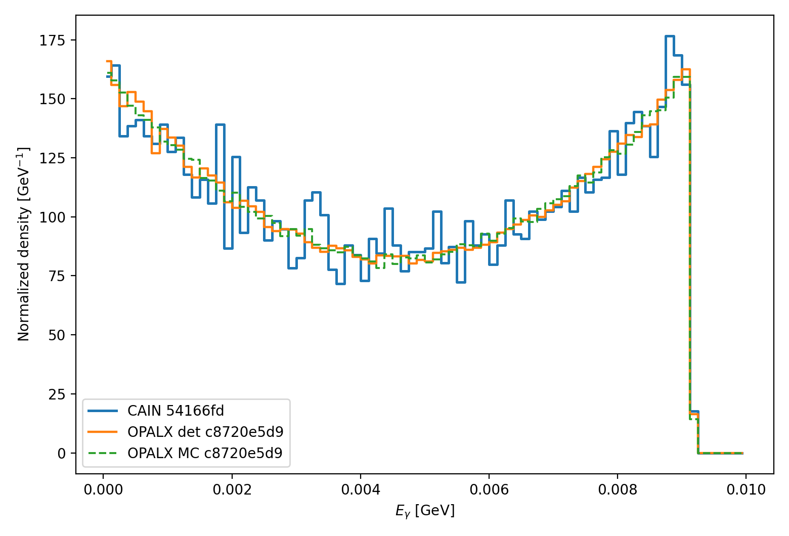
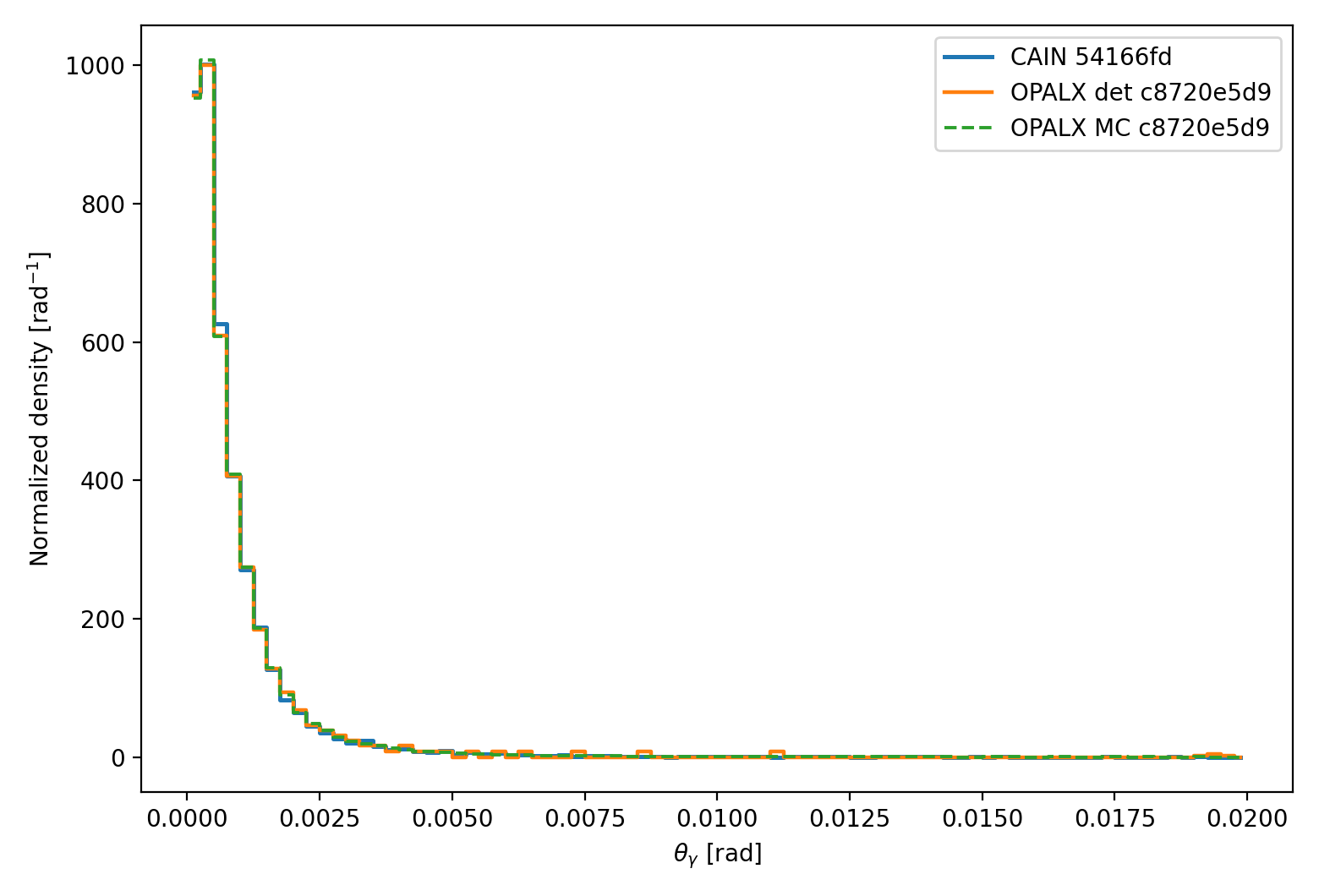
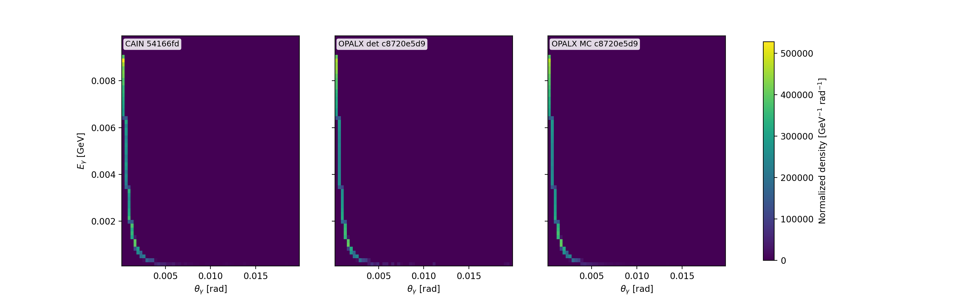
9.2.4 Results of Code Comparison
The current CAIN-backed OPALX benchmark covers weak-field linear inverse Compton scattering for:
electron total energy
1GeV,laser wavelength
1030nm,crossing angle \(90^\circ\),
unpolarized laser
STOKES=(0,0,0),CAIN weak-field parameter \(\xi = 0.2955 < 0.3\).
Single-electron benchmark agreement:
Finite-beam benchmark agreement:
Single-electron overlays:
Finite-beam overlays:


9.2.5 Build and Run
The CAIN build helper is now shared across the gamma-gamma notes in the common workspace ~/git/cain.
From ~/git/cain:
./build-cain.sh --download
./build-cain.sh --compile
The preferred one-shot workflow is run from the docs tree:
cd ~/git/OPALX-project.github.io/gamma-gamma
./generate-gamma-gamma-results.sh --opalx-build /path/to/opalx-laser/build_openmp
This top-level driver:
builds the OPALX gamma-gamma benchmark targets,
runs the inverse-Compton and Breit-Wheeler unit/regression suites,
regenerates the CAIN and OPALX benchmark data for both notes,
republishes the comparison figures, and
renders the gamma-gamma note pages.
If only the linear-Compton assets need to be refreshed, use:
cd ~/git/cain
./generate-linear-compton-results.sh --opalx-build /path/to/opalx-laser/build_openmp
This script:
runs the CAIN decks
~/git/cain/cain-linear-compton-90deg.i,~/git/cain/cain-linear-compton-90deg-finite-beam.i,~/git/cain/cain-linear-compton-90deg-finite-beam-energy-spread.i, and~/git/cain/cain-linear-compton-90deg-finite-beam-overlap.i,regenerates the stored CAIN histogram references in
figures/reference-data/,runs the OPALX benchmark executable
LinearComptonSpectrumBenchmark,regenerates the published 1D and 2D comparison plots in
figures/reference-data/.
The script expects:
a built OPALX benchmark executable in the supplied build directory,
a CAIN executable at
~/git/cain/CAIN-build/cain, unless overridden by--cain-bin,the four CAIN decks in
~/git/cain, unless overridden by--cain-deck-dir.
The relevant OPALX build target is:
cmake --build /path/to/opalx-laser/build_openmp \
  --target LinearComptonSpectrumBenchmark TestLinearCompton TestLinearComptonSpectrum -j4
9.2.6 References
CAIN linear Compton generator:
src/lncpgn.fCAIN laser geometry helper:
src/lsrgeo.fCAIN manual: User’s Manual of CAIN
9.2.7 CAIN Mapping
CAIN evaluates the linear Compton kinematics by boosting the laser photon into the electron rest frame, applying the recoil there, and boosting the scattered photon back to the laboratory frame. In CAIN’s LNCPGN, the incoming photon energy in the electron rest frame is
\[ \omega_1 = \gamma \, \omega_L \, (1 - \beta \cos \alpha) . \tag{9.8}\]
For the present benchmark \(\cos\alpha = 0\), so
\[ \omega_1 = \gamma \, \omega_L . \tag{9.9}\]
This is the CAIN mapping reproduced by the current OPALX helper and benchmark path.
9.3 Breit-Wheeler Theory
9.3.1 Scope
This note describes the minimum Breit-Wheeler physics model needed for the next OPALX benchmark.
We follow closely the CAIN ansatz i.e. manual and source code.
The goal is not yet a full tracking implementation. The immediate target is a host-side Monte Carlo and deterministic benchmark path that reproduces CAIN for the process
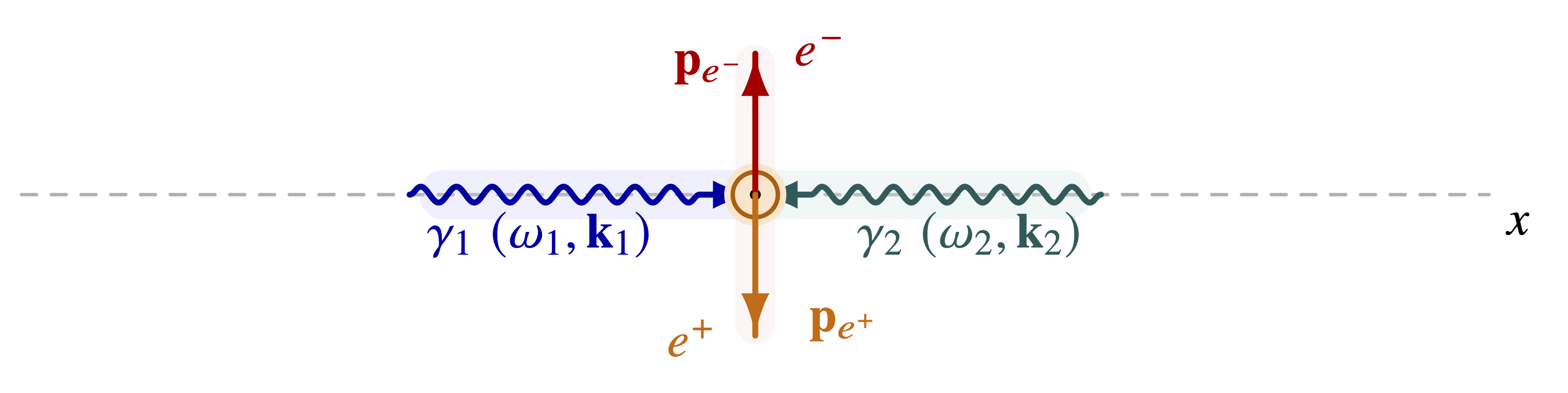
\[\gamma + \gamma \rightarrow e^- + e^+ .\]
The first benchmark will follow the same strategy as the linear ICS work:
start from a fixed-geometry, unpolarized, linear process;
implement the core event kernel in;
validate deterministic and sampled spectra against CAIN;
delay bunch population and tracker integration until the kernel is trusted.
9.3.2 Linear Breit-Wheeler Kinematics in CAIN
CAIN’s linear generator LNBWGN uses two incoming photons:
a laser photon with energy \(W_1\) and direction \(\mathbf{n}_1\),
a high-energy photon with energy \(W_2\) and direction \(\mathbf{n}_2\).
Note: in a collider setup the laser photon is also a high-energy photon.
The opening-angle dependence enters through
\[Z_0 = \mathbf{n}_1 \cdot \mathbf{n}_2 .\]
The two-photon invariant used in CAIN is
\[ S_0 = 2 W_1 W_2 (1 - Z_0) . \tag{9.10}\]
Pair creation is kinematically allowed only if
\[ S_0 \ge 4 m_e^2 . \tag{9.11}\]
This threshold appears directly in LNBWGN:
S0=2*W1*W2*(1-Z0)
IF (4*M**2.GT.S0) GOTO 900
In a head-on geometry, \(Z_0 = -1\), so the threshold reduces to
\[ W_1 W_2 \ge m_e^2 . \tag{9.12}\]
This is the cleanest geometry for the first benchmark.
CAIN constructs the center-of-momentum boost velocity from the two incoming photon momenta and then samples the final-state scattering variables in that frame.
The code introduces a transformed photon energy \(W\) and several auxiliary variables:
\[ W = \gamma W_1 V_R, \qquad X = \frac{\sqrt{W^2 - m_e^2}}{W}, \qquad X_1 = \frac{m_e^2}{W^2 + W\sqrt{W^2 - m_e^2}} . \tag{9.13}\]
The random variable \(Y\) is used to generate the CM scattering angle through
\[ \cos\theta = 1 - 2Y . \tag{9.14}\]
The resulting Mandelstam-like combinations in the CAIN implementation are
\[ s_m = \frac{2m_e^2}{(1+X)X_1}\left[X(1-2Y)-1\right], \qquad u_m = -\frac{2m_e^2}{(1+X)X_1}\left[X(1-2Y)+1\right] . \tag{9.15}\]
CAIN then builds the angular kernel from
\[ \cos\theta_1 = 1 + 2m_e^2\left(\frac{1}{u_m} + \frac{1}{s_m}\right) \tag{9.16}\]
and
\[ D = -\left(\frac{s_m}{u_m} + \frac{u_m}{s_m}\right) . \tag{9.17}\]
For unpolarized incoming photons, the acceptance weight reduces to the unpolarized part of the full CAIN expression.
9.3.3 OPALX Validation Path
Deterministic physics helper
Host-only sampled event generator
no tracker, no photon bunch population, no GPU path yet
CAIN comparison
9.3.4 Implemented OPALX Benchmark
The current OPALX implementation is documented in the local Doxygen build. The relevant pages are:
~/git/cain/linear-breit-wheeler-head-on.i~/git/cain/generate-linear-breit-wheeler-results.sh
The benchmark remains deliberately narrow:
no tracker integration,
no bunch population,
no GPU path.
The validated observables are now:
Finite incoming-photon-beam benchmark:
The finite-photon-beam extension is still intentionally narrow:
the high-energy photon beam is sampled only in momentum space,
the reference beam axis is the head-on direction,
the angular spread is Gaussian with \(\sigma_{\theta x} = \sigma_{\theta y} = 1\,\mathrm{mrad}\),
the current published benchmark keeps the photon-beam relative energy spread at zero,
there is still no transverse position spread or laser-overlap weighting in the OPALX benchmark path.
Local Kernel Tests
The current OPALX implementation now exposes the same proposal-coordinate view used by the CAIN rejection sampler. Two helper functions are validated directly in the unit tests:
the map from the proposal variable \(z \in [-1,1\)] to the center-of-momentum scattering cosine \(\cos\theta\),
the corresponding unpolarized local angular weight in the same proposal coordinate.
This gives a direct check of the differential kernel itself, not only of its integrated or sampled consequences. The pointwise tests use an independent reference implementation of the CAIN-aligned auxiliary variables \(Y(z)\), \(s_m\), \(u_m\), and the local acceptance weight.
Finite-Photon-Beam Folding Algorithm
For the finite incoming-photon-beam benchmark, OPALX keeps the laser photon fixed and samples only the high-energy photon beam. For each event:
a high-energy photon direction is drawn from a Gaussian angular spread around the head-on reference axis,
the photon energy is either kept fixed or, in the extended code path, drawn from a Gaussian relative energy spread,
a per-event linear Breit-Wheeler sampling kernel is built from that sampled incoming photon state and the fixed laser photon,
the electron-positron event is generated with the same host-side rejection sampler used in the fixed-geometry benchmark,
the requested observable is histogrammed and compared to the matching CAIN reference.
The present published finite-photon-beam result validates only the divergence broadening. The next benchmark extensions are:
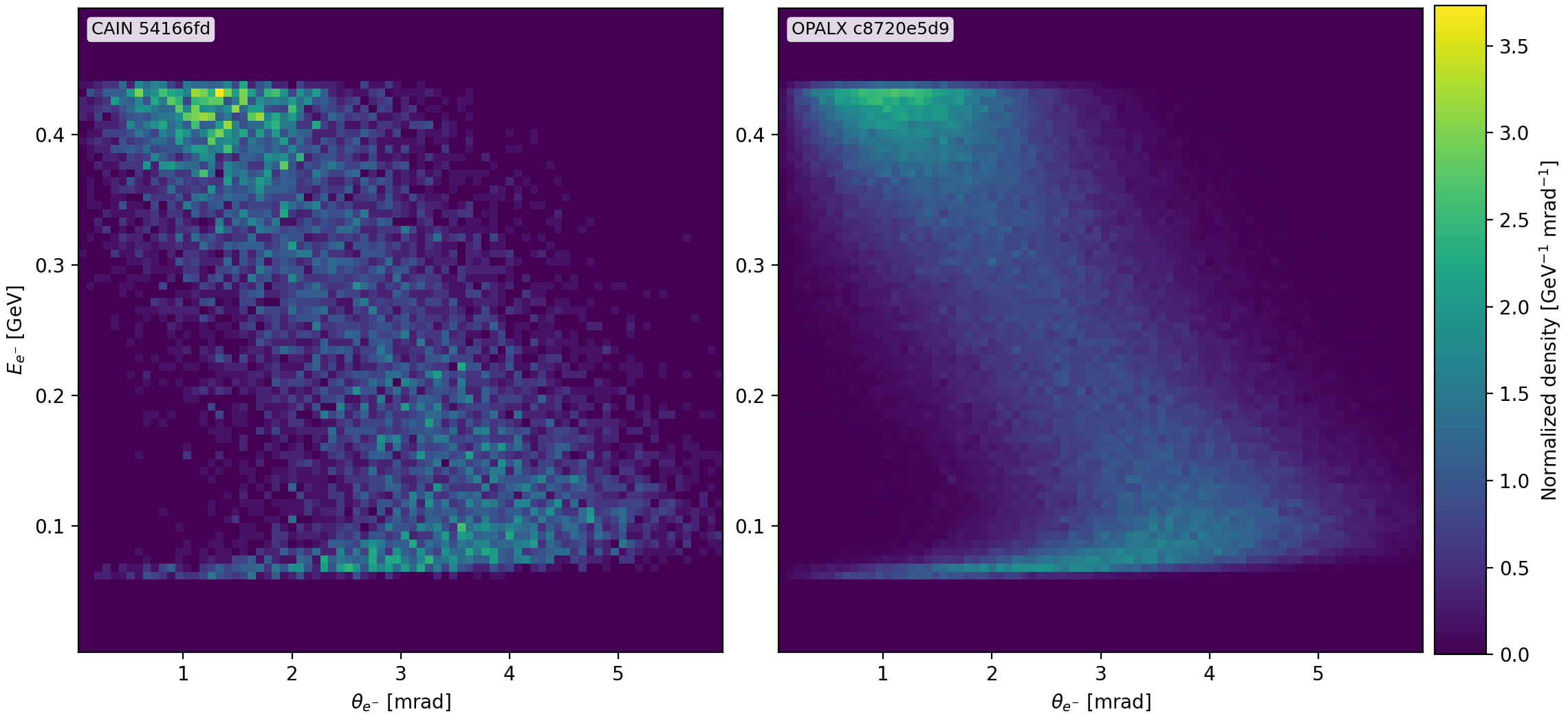
joint \(E\)--\(\theta\) maps for the finite incoming photon beam,
finite-photon-beam benchmarks with nonzero photon-beam relative energy spread.
9.3.5 Results of Code Comparison
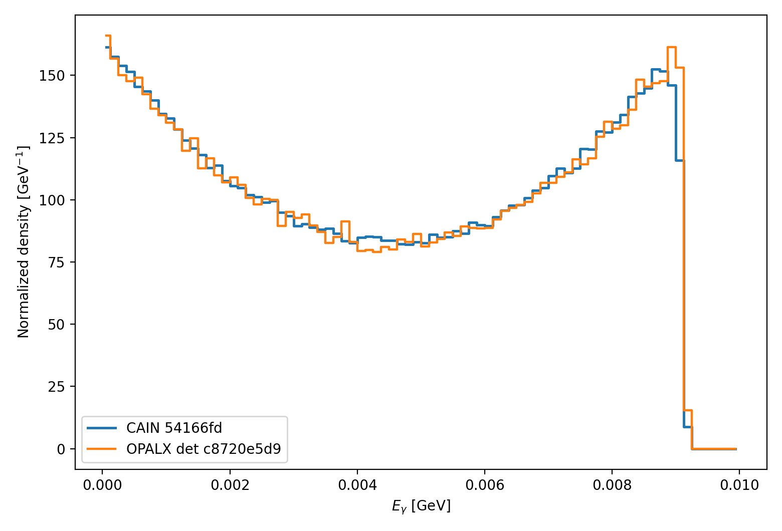
The current CAIN-backed OPALX benchmark compares the linear unpolarized process LASERQED BREITWHEELER, NPH=0 for a weak-field setup with \(\xi = 0.25\). The benchmark observables are:
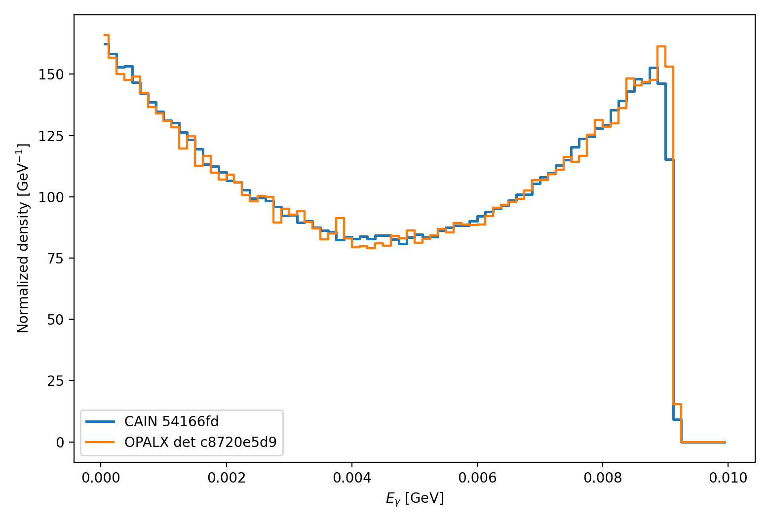
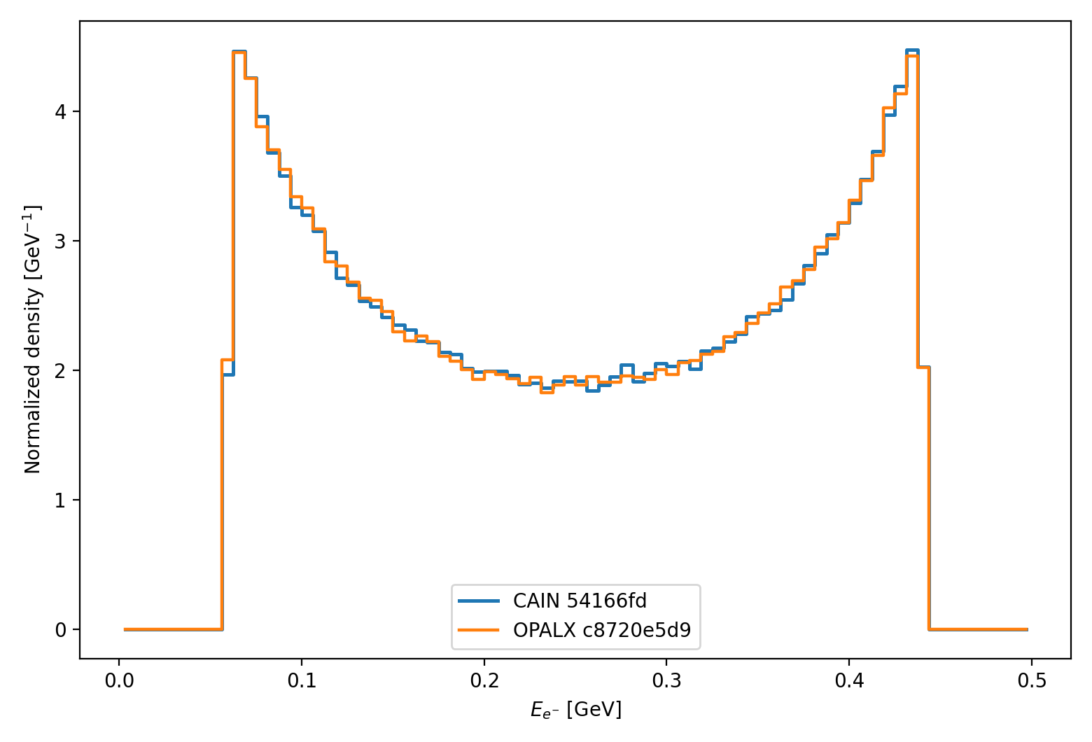
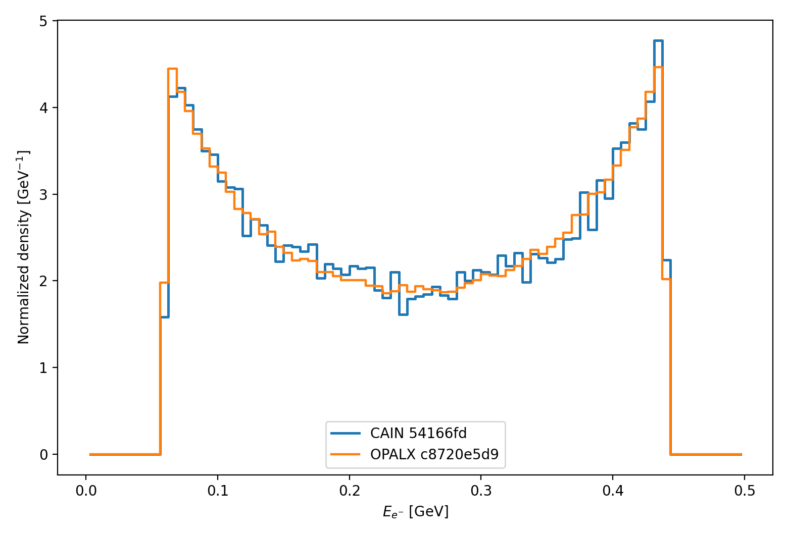
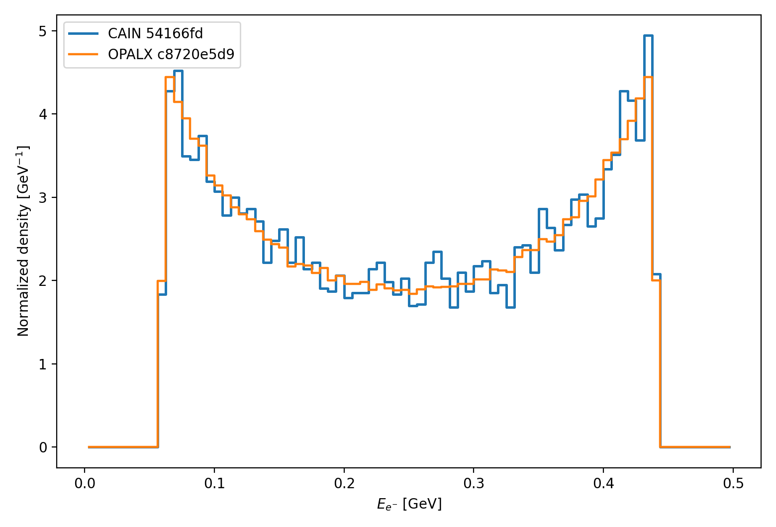
electron energy spectrum,
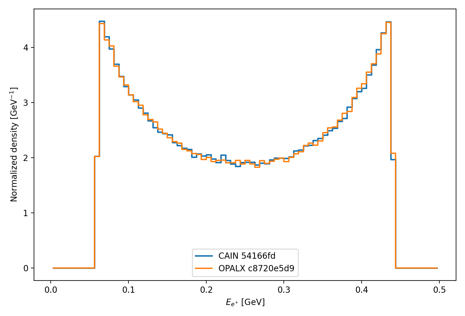
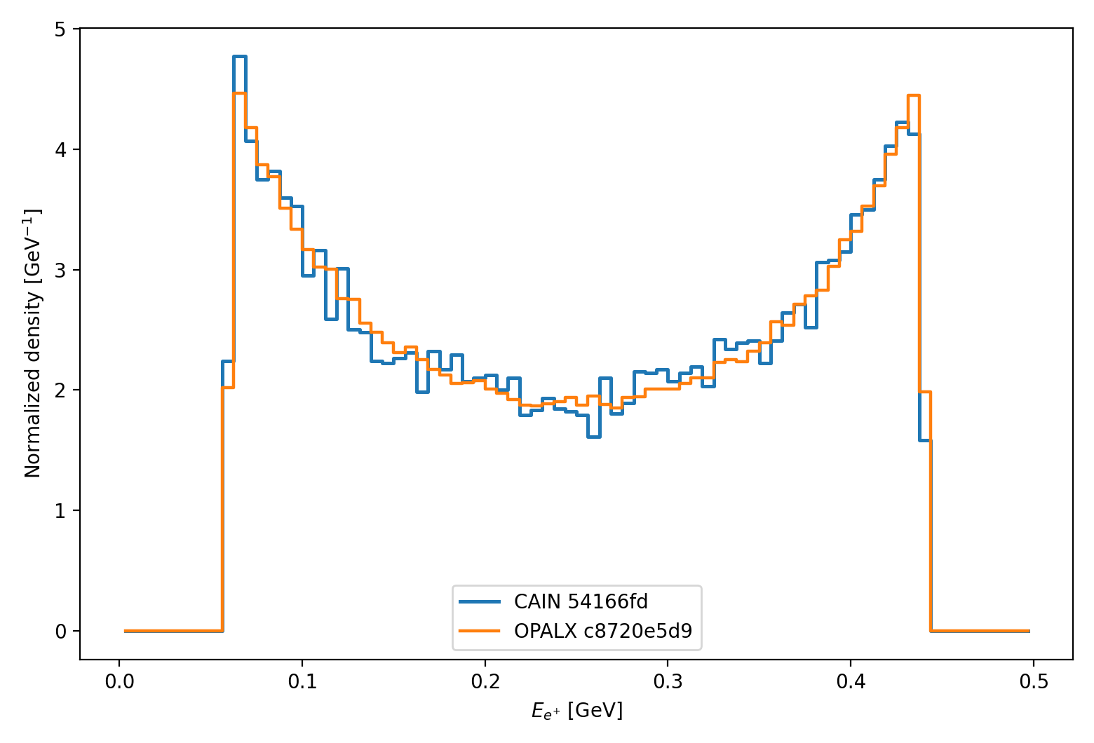
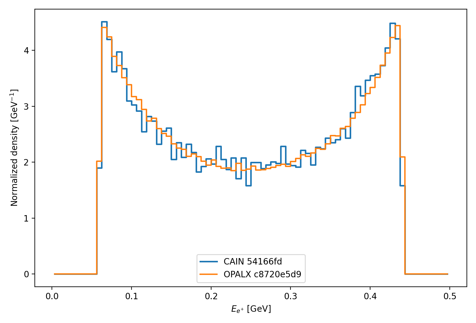
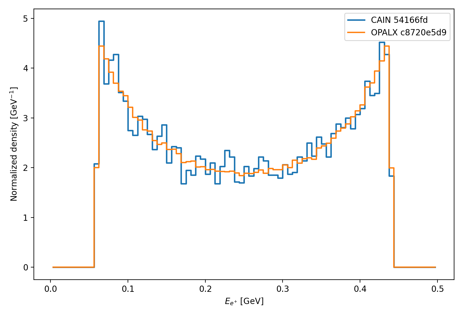
positron energy spectrum,
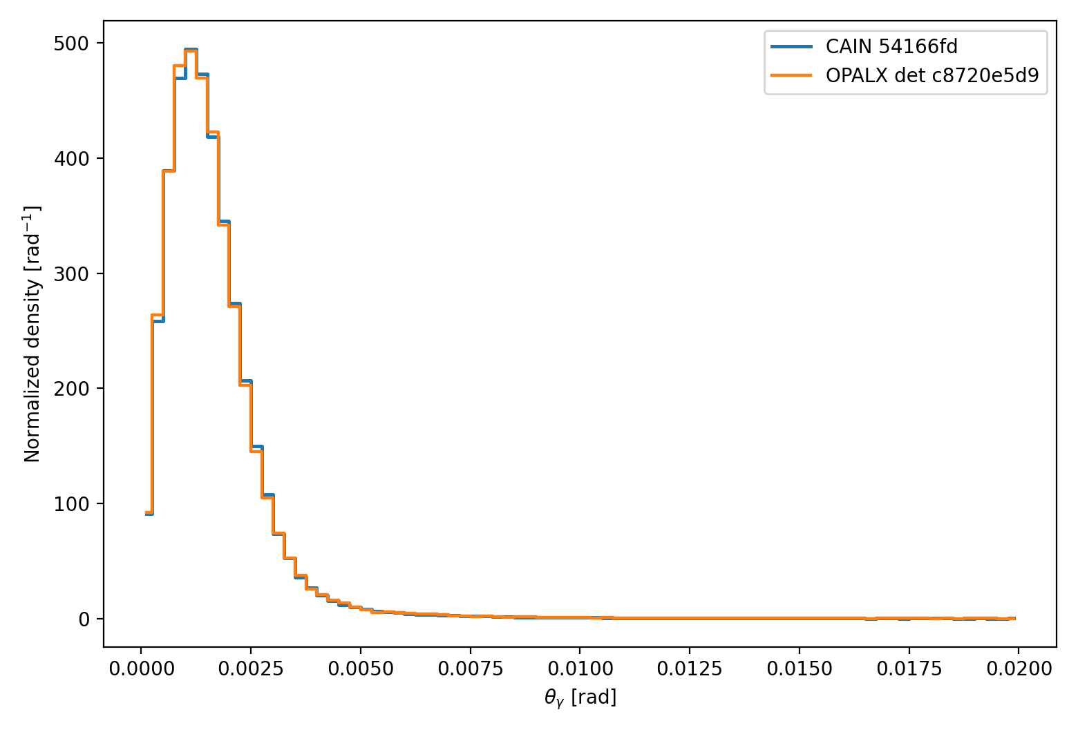
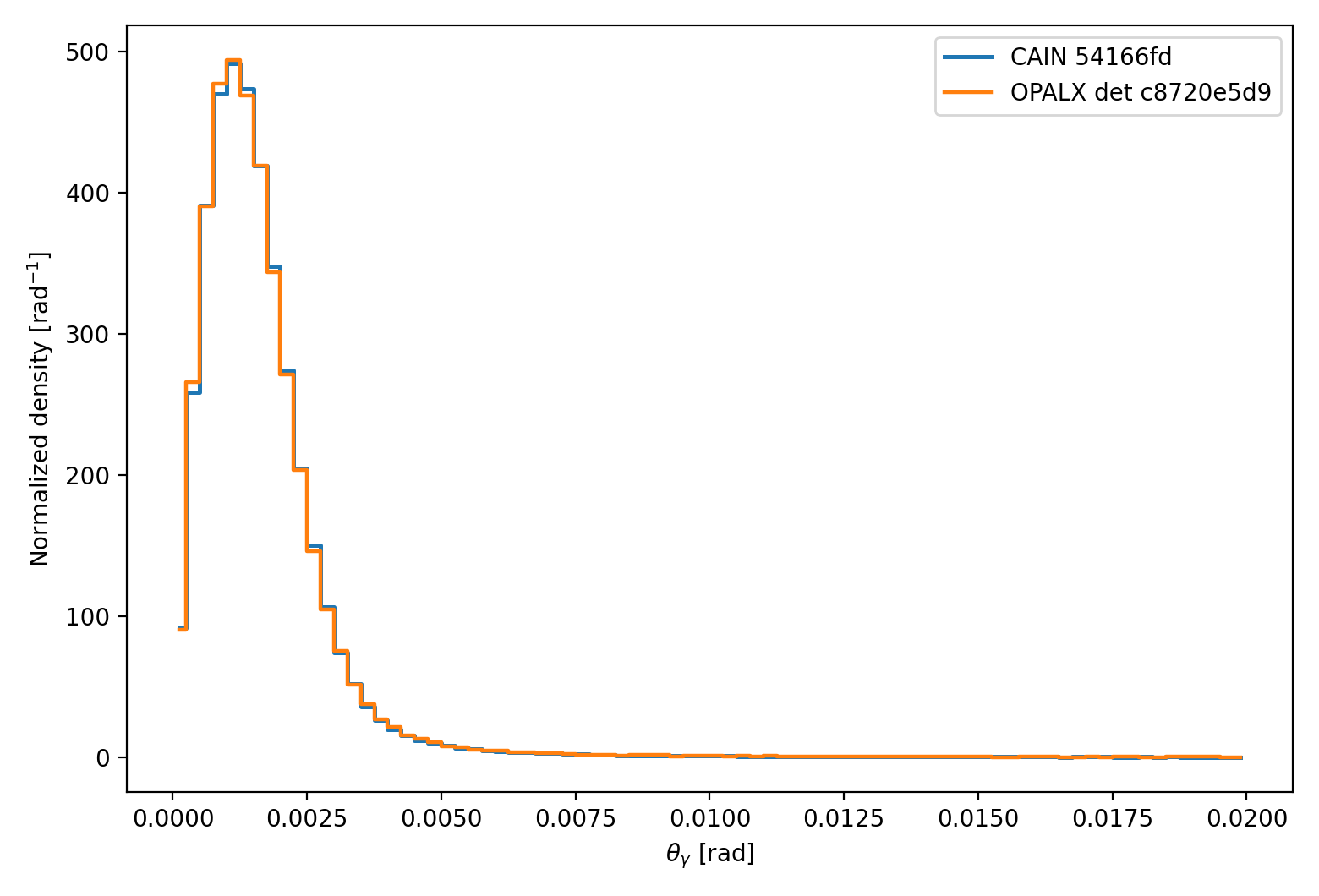
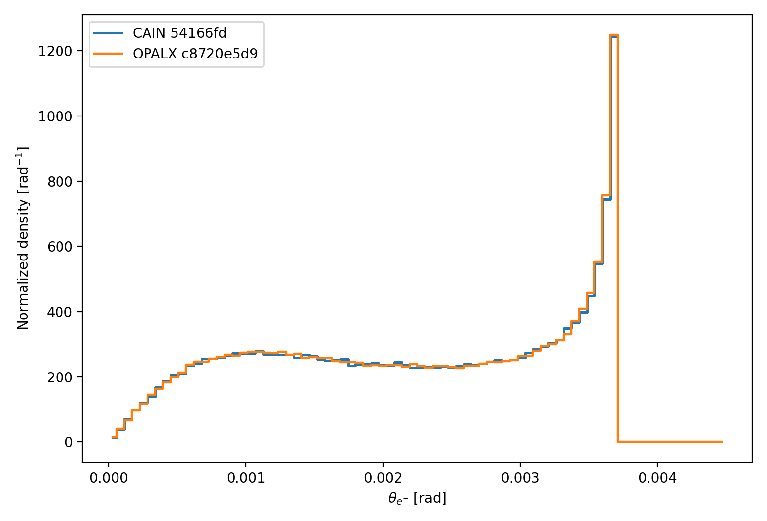
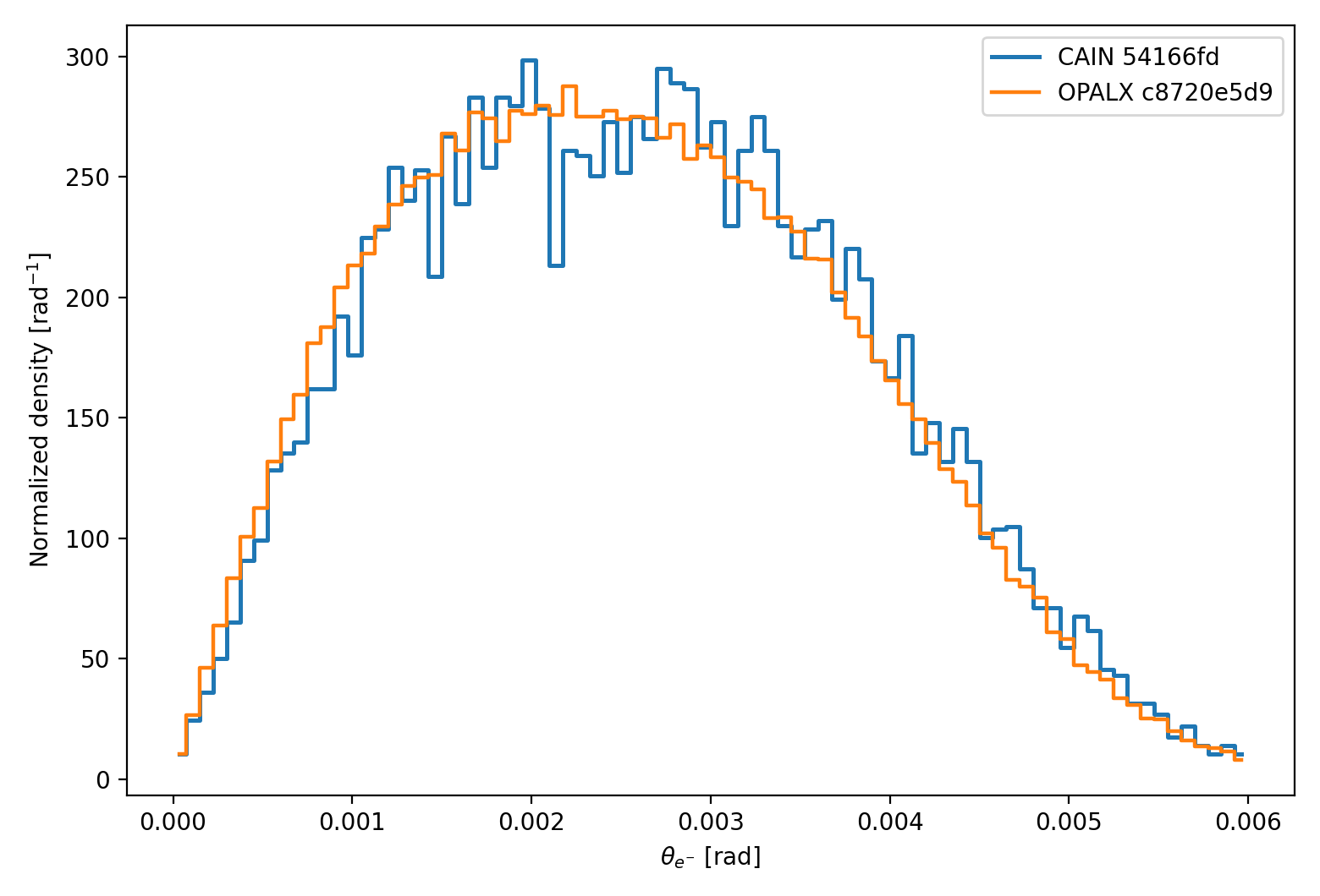
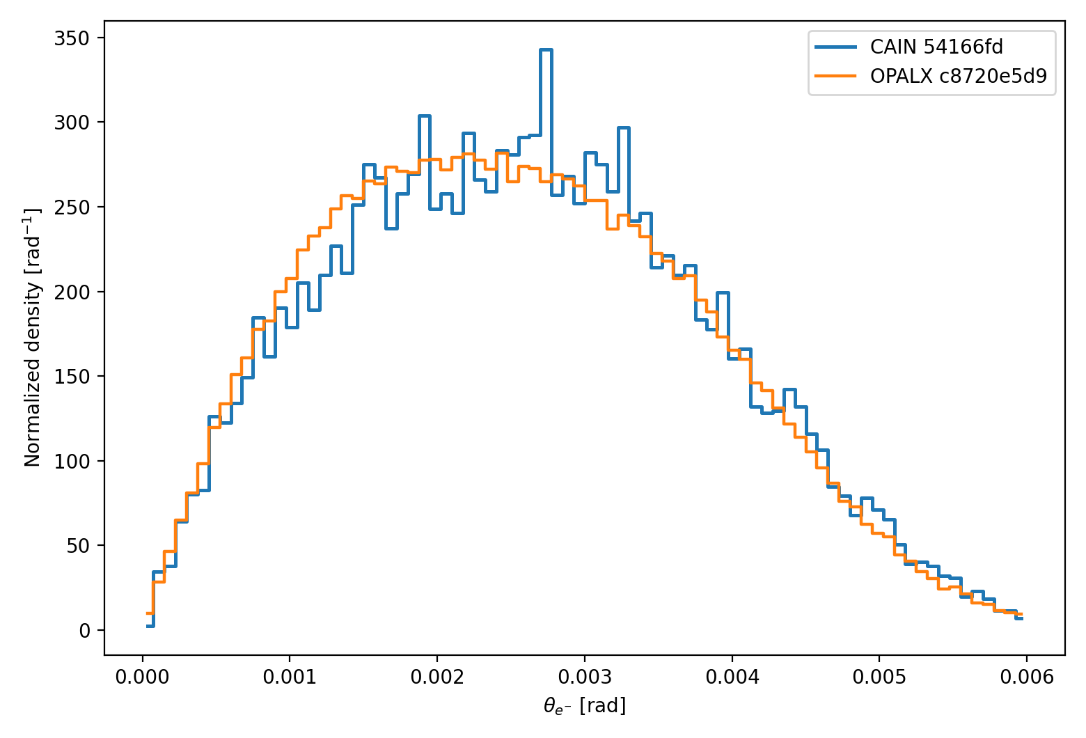
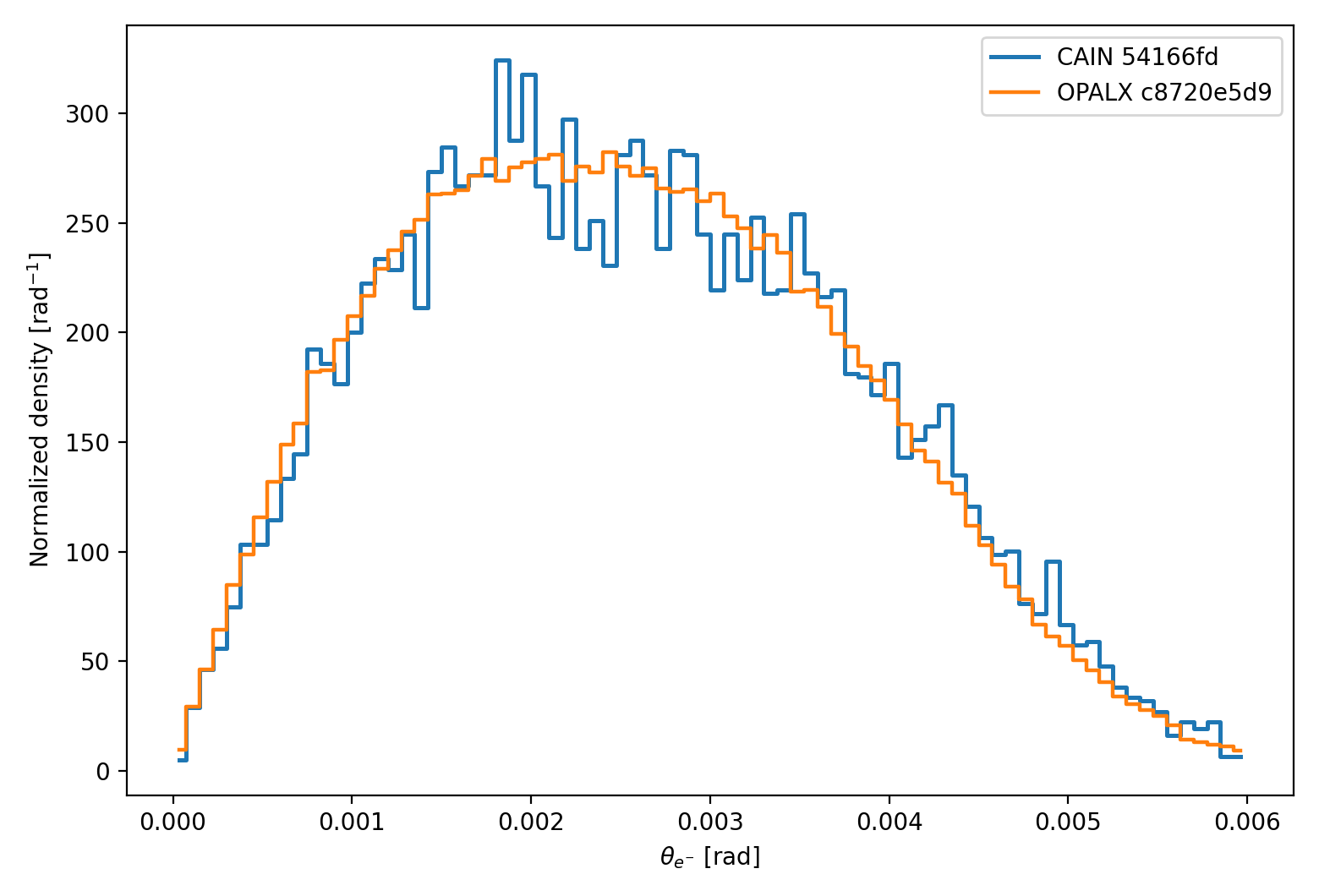
electron angle spectrum,
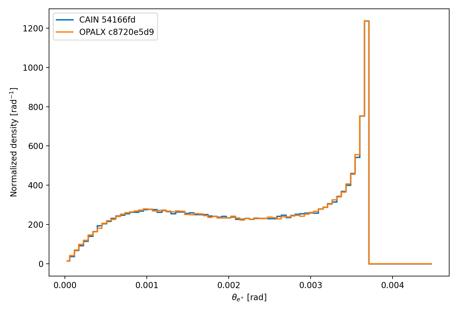
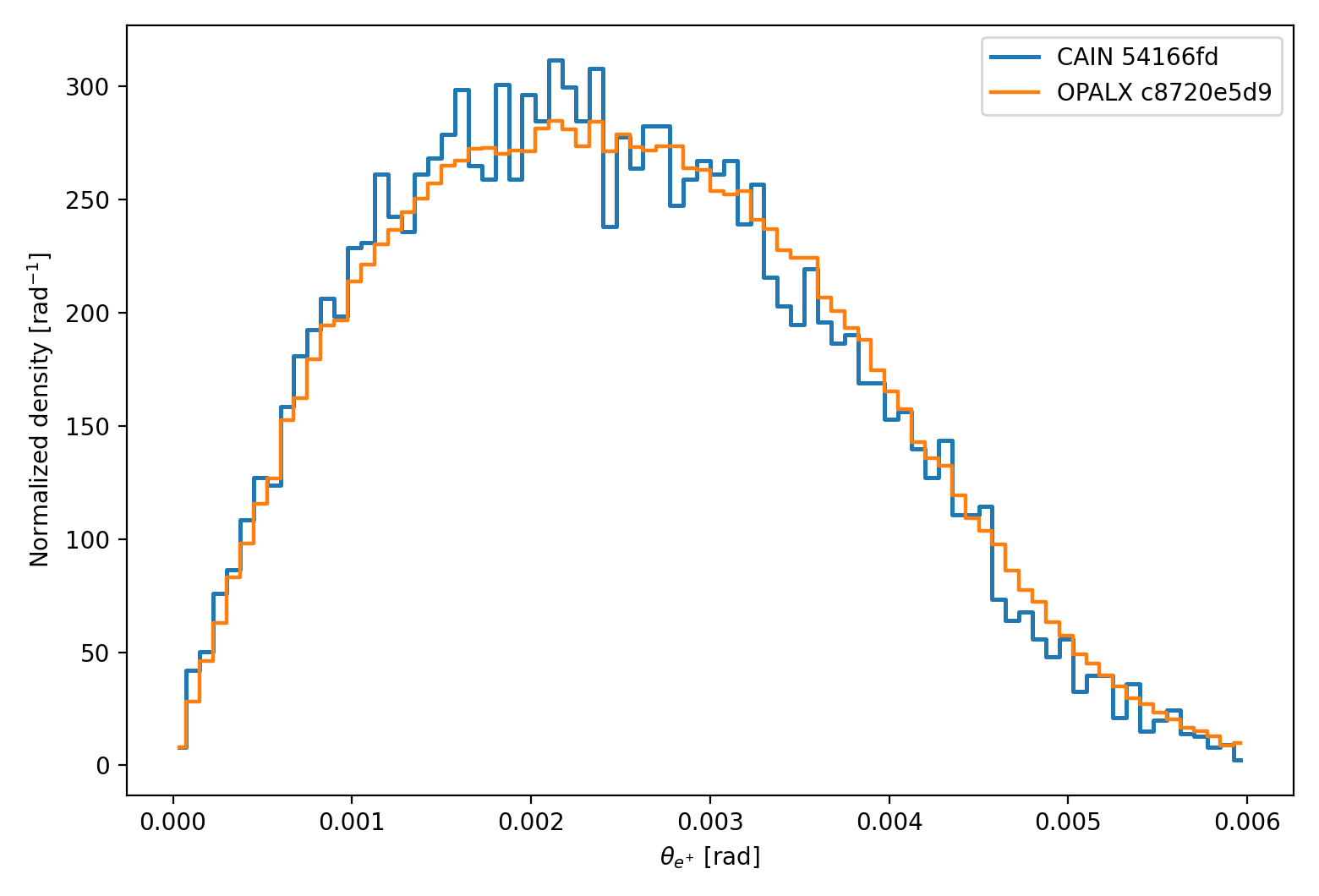
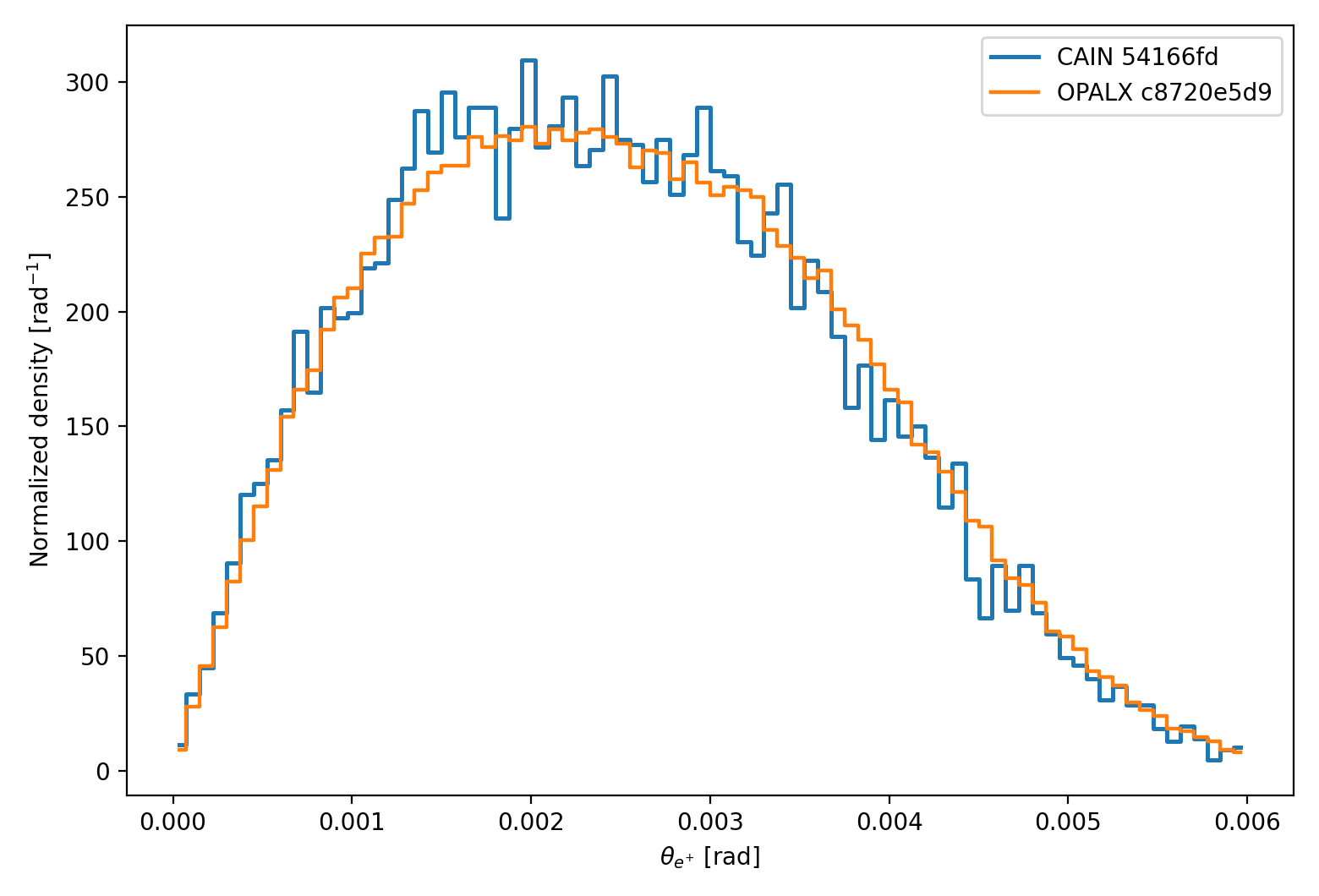
positron angle spectrum,
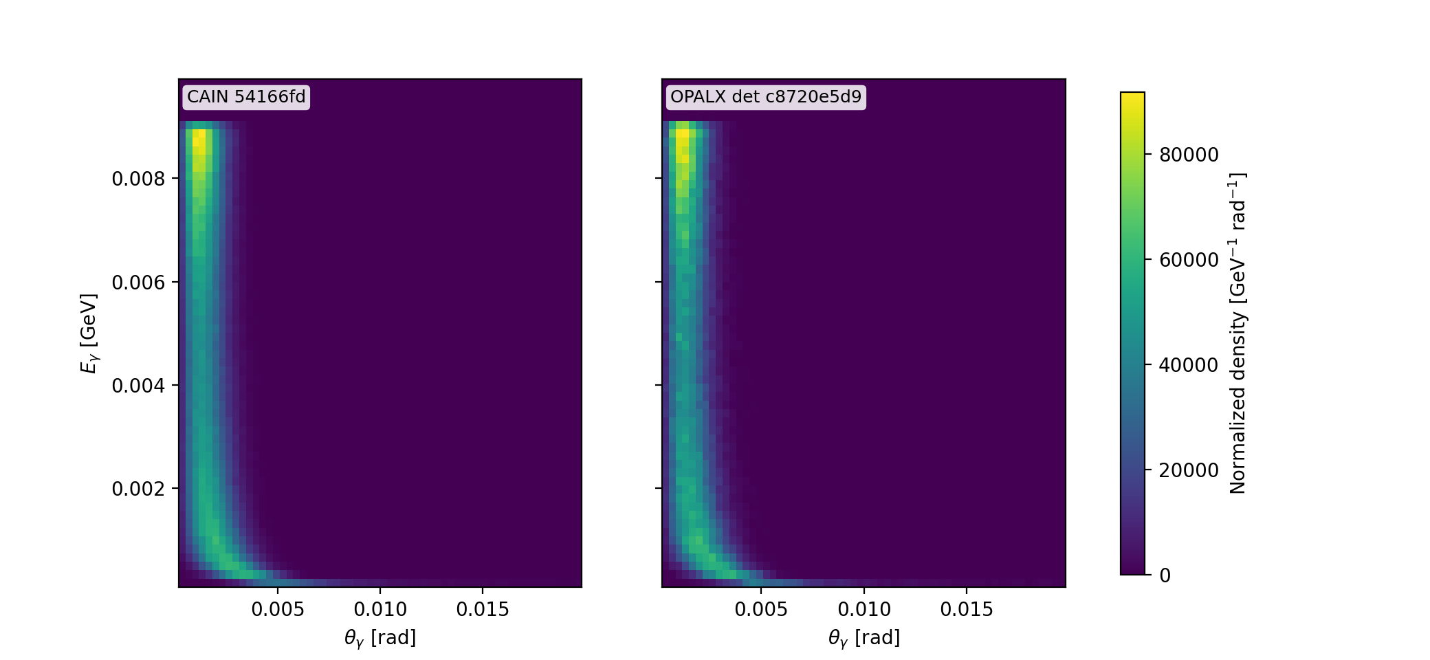
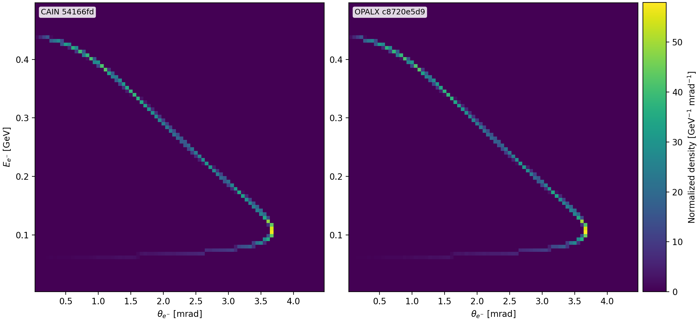
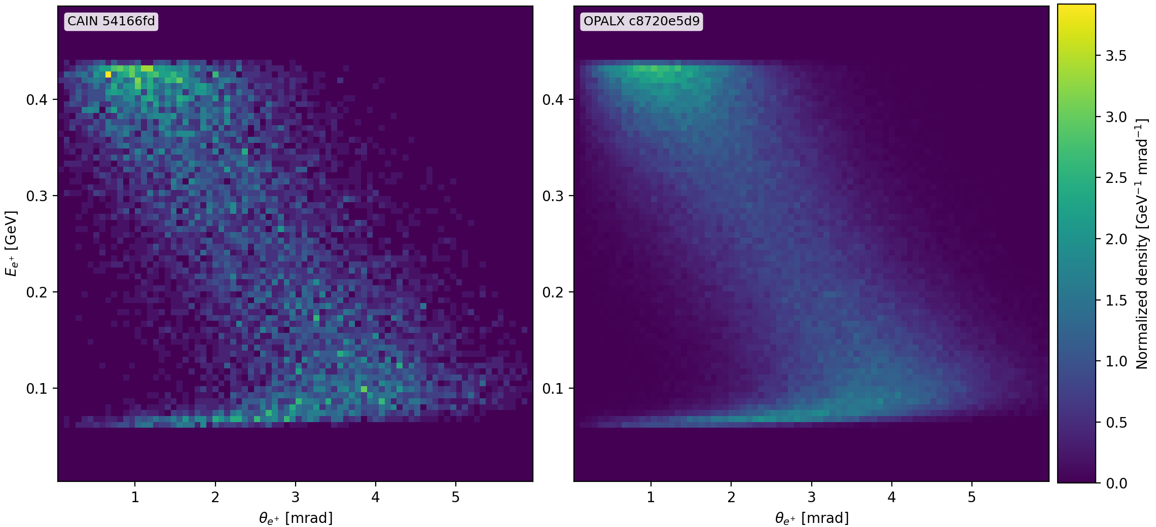
joint \(E\) vs. \(\theta\) maps for electron and positron,
and, in the extended benchmark, the same 1D observables for a finite incoming photon beam.
The first fixed-geometry comparison point uses:
head-on geometry,
\(E_\gamma = 0.5\,\mathrm{GeV}\),
\(\lambda_L = 1\,\mathrm{nm}\),
unpolarized photons.
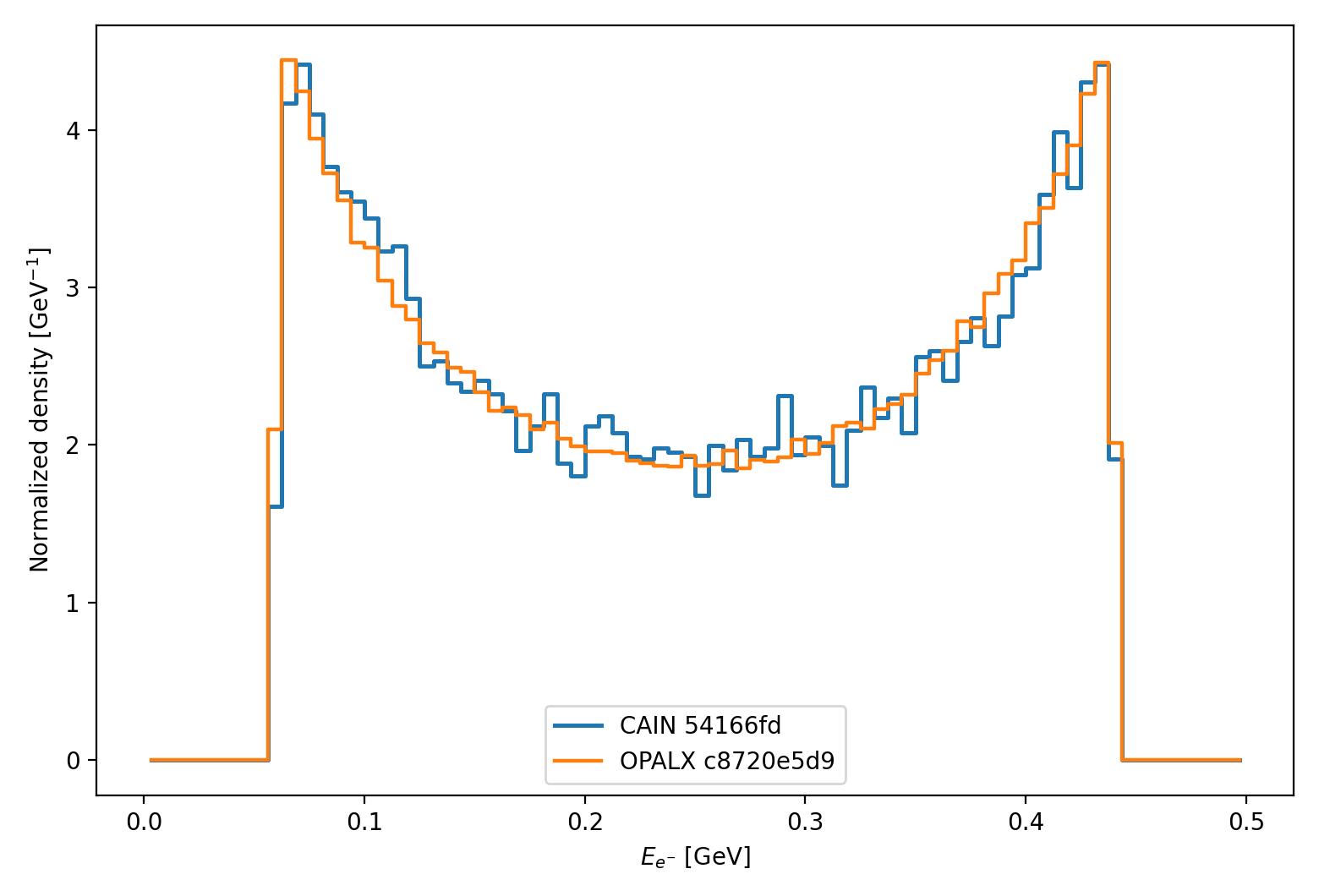
With the current OPALX Monte Carlo benchmark and the stored CAIN references, the agreement is already tight.
Electron:
Positron:
So the present benchmark already supports both 1D and 2D CAIN-backed regression coverage for the linear unpolarized kernel.
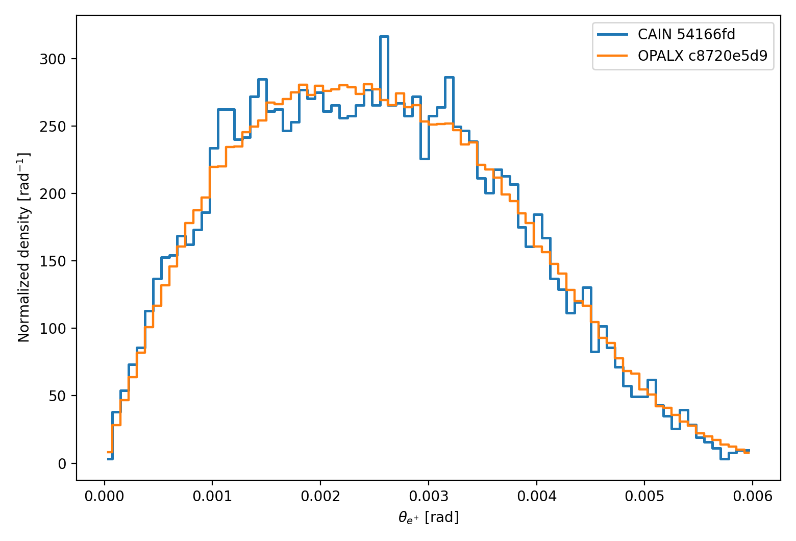
Finite incoming-photon-beam point:
head-on reference geometry,
\(E_\gamma = 0.5\,\mathrm{GeV}\),
\(\lambda_L = 1\,\mathrm{nm}\),
Gaussian photon-beam divergence with \(\sigma_{\theta x} = \sigma_{\theta y} = 1\,\mathrm{mrad}\),
zero photon-beam energy spread.
Finite-photon-beam agreement:
Electron:
Positron:
Finite-photon-beam plus energy-spread agreement:
Electron:
Positron:
The finite-photon-beam angle benchmarks are intentionally windowed to \(0 \le \theta \le 6\,\mathrm{mrad}\), so the stored CAIN angular histograms do not integrate to exactly one inside that clipped range.
The fixed-geometry head-on comparisons are shown for the electron in Figure 9.12, Figure 9.13, and Figure 9.14, and for the positron in Figure 9.23, Figure 9.24, and Figure 9.25.
The finite-photon-beam comparisons with Gaussian divergence and zero energy spread are shown for the electron in Figure 9.15, Figure 9.16, and Figure 9.17, and for the positron in Figure 9.26, Figure 9.27, and Figure 9.28.
The finite-photon-beam plus energy-spread comparisons are shown for the electron in Figure 9.18, Figure 9.19, and Figure 9.20, and for the positron in Figure 9.29, Figure 9.30, and Figure 9.31.
The overlap-restricted comparisons are shown for the electron in Figure 9.21 and Figure 9.22, and for the positron in Figure 9.32 and Figure 9.33.


9.3.6 Build and Run
The preferred one-shot workflow is run from the docs tree:
cd ~/git/OPALX-project.github.io/gamma-gamma
./generate-gamma-gamma-results.sh \
  --opalx-build ~/git/opalx-laser/build_openmp
This top-level driver:
builds the OPALX gamma-gamma benchmark targets,
runs the inverse-Compton and Breit-Wheeler unit/regression suites,
regenerates the CAIN and OPALX benchmark data for both notes,
republishes the comparison figures, and
renders the gamma-gamma note pages.
If only the Breit-Wheeler assets need to be refreshed, use:
cd ~/git/cain
./generate-linear-breit-wheeler-results.sh \
  --opalx-build ~/git/opalx-laser/build_openmp
This script:
runs the CAIN decks
~/git/cain/linear-breit-wheeler-head-on.i,~/git/cain/linear-breit-wheeler-finite-photon-beam.i,~/git/cain/linear-breit-wheeler-finite-photon-beam-energy-spread.i, and~/git/cain/linear-breit-wheeler-overlap.i,regenerates the stored CAIN histogram references in
~/git/opalx-laser/unit_tests/Physics/data,runs the OPALX benchmark executable
LinearBreitWheelerBenchmarkfor fixed-geometry, finite-photon-beam, finite-photon-beam-plus-energy-spread, and overlap cases,regenerates the 1D and 2D comparison plots in
~/git/cain/reference-data.
The script expects:
a built OPALX benchmark executable in the supplied build directory,
a CAIN executable at
~/git/cain/CAIN-build/cain, unless overridden by--cain-bin.
The relevant unit-test targets are:
cmake --build ~/git/opalx-laser/build_openmp \
  --target TestLinearBreitWheeler TestLinearBreitWheelerSpectrum LinearBreitWheelerBenchmark -j4

~/git/opalx-laser/build_openmp/unit_tests/Physics/TestLinearBreitWheeler
~/git/opalx-laser/build_openmp/unit_tests/Physics/TestLinearBreitWheelerSpectrum
9.3.7 References
CAIN source parser:
src/rdlqed.fCAIN Breit-Wheeler runtime loop:
src/lsrqedbw.fCAIN linear Breit-Wheeler generator:
src/lnbwgn.fCAIN nonlinear Breit-Wheeler generator:
src/nlbwgn.fCAIN weighted event insertion:
src/lbwevent.fCAIN manual: User’s Manual of CAIN
9.3.8 CAIN Structure
CAIN separates Breit-Wheeler physics into three layers.
Input and model selection
LASERQEDBREITWHEELERis parsed insrc/rdlqed.f.NPH=0selects the linear Breit-Wheeler model.NPH>=1selects the nonlinear model.
Runtime driver
The laser-particle loop is handled by
src/lsrqedbw.f.Local laser geometry and power density are obtained from
LSRGEO.The linear event generator is
LNBWGN.The nonlinear event generator is
NLBWGN.If an event happens, the produced electron and positron are inserted by
LBWEVENT.
Event generation
Linear Breit-Wheeler:
src/lnbwgn.fNonlinear Breit-Wheeler:
src/nlbwgn.fWeighted particle insertion:
src/lbwevent.f
For the first OPALX benchmark only the linear event kernel is needed.