3  Elements

This chapter documents element models whose geometry, field support, or runtime semantics require more than the generic placement conventions.

3.1 Analytic sector and rectangular bends

The current OPALX-native analytic SBEND and RBEND implementation is a field-based bend model with explicit body placement, explicit field-support extent, and first-order fringe optics. The implementation does not replace bend tracking by transfer matrices. Instead, the reference particle and the bunch are integrated through the magnetic field that is evaluated in the local bend chart.

3.1.1 Body extent and field-support extent

The nominal body extent is the placed hardware interval \[ z \in [0, L], \] where (L) is the body length used for placement, body ports, and geometry export.

The field-support extent may extend beyond the body through entry and exit fringe regions, \[ z \in [-\ell_{\mathrm{entry}},\, L + \ell_{\mathrm{exit}}], \] with \[ \ell_{\mathrm{entry}} = \frac{h_{\mathrm{gap}} F_{\mathrm{int}}}{|\cos E_1|}, \qquad \ell_{\mathrm{exit}} = \frac{h_{\mathrm{gap}} F_{\mathrm{int}}}{|\cos E_2|}. \] Here (h_{}) is the half gap (HGAP), (F_{}) is the fringe integral (FINT), and (E_1), (E_2) are the entrance and exit pole-face angles. If HGAP is not given, OPALX uses the fallback \[ h_{\mathrm{gap}} = \frac{\mathrm{GAP}}{2}. \]

The body extent drives placement and visualization. The field-support extent drives field evaluation, active-set occupancy, and timestep sanity checks. This is why OPALX can export both body markers (ENTRY EDGE, EXIT EDGE) and field-support markers (FIELD BEGIN, FIELD END) for the same bend.

3.1.2 Effective field length and bend normalization

The implemented fringe-support model uses a linear hard-edge ramp at both faces. The effective field length is therefore defined as \[ L_{\mathrm{eff}} = L_{\mathrm{ref}} + \frac{\ell_{\mathrm{entry}} + \ell_{\mathrm{exit}}}{2}, \] where (L_{}) is the body length measured along the design reference path.

For SBEND, the design reference-path body length equals the sector-bend body length, \[ L_{\mathrm{ref}}^{\mathrm{SBEND}} = L. \] For RBEND, the design reference-path body length is the curved reference-path length between the rotated entrance and exit faces, \[ L_{\mathrm{ref}}^{\mathrm{RBEND}} = L_{\mathrm{arc}}, \] not the straight body chord. This distinction is required to normalize the analytic rectangular-bend field on the actual design orbit rather than on the mechanical chord.

ANGLE is the primary geometric input. The analytic dipole coefficient is normalized against the effective field length, \[ k_0 = \frac{\theta}{L_{\mathrm{eff}}}, \] with total bend angle (). K0 is treated only as a secondary consistency-check quantity.

Internally, OPALX stores the analytic bend strengths in normalized lattice form and converts them to physical Tesla coefficients only when a reference rigidity is available. If DESIGNENERGY is given, that kinetic energy is used together with the bunch species mass and charge. Otherwise the scaling is taken from the bunch reference momentum. This avoids tying bend tracking strength to the parser-global quantity (P_0).

3.1.3 Longitudinal field profile

The body field is multiplied by a longitudinal scale function ((z)) defined by \[ \lambda(z) = \begin{cases} 0, & z < -\ell_{\mathrm{entry}}, \\ \dfrac{z + \ell_{\mathrm{entry}}}{\ell_{\mathrm{entry}}}, & -\ell_{\mathrm{entry}} \le z \le 0, \\ 1, & 0 \le z \le L, \\ \dfrac{L + \ell_{\mathrm{exit}} - z}{\ell_{\mathrm{exit}}}, & L \le z \le L + \ell_{\mathrm{exit}}, \\ 0, & z > L + \ell_{\mathrm{exit}}. \end{cases} \]

This is a field-support model, not a body-length remapping. Particles begin to see the bend field at FIELD BEGIN, not necessarily at ENTRY EDGE.

3.1.4 First-order fringe optics

In addition to the longitudinal field ramp, the implementation includes a first-order edge-focusing model. With signed curvature \[ h = \frac{\theta}{L_{\mathrm{eff}}}, \] the horizontal hard-edge relation is \[ x'_{\mathrm{out}} = x'_{\mathrm{in}} + h \tan(E)\,x. \]

The vertical edge focusing includes the standard fringe correction \[ \psi = h\,h_{\mathrm{gap}}\,F_{\mathrm{int}} \frac{1 + \sin^2(E)}{\cos(E)}, \] so the implemented vertical law is \[ y'_{\mathrm{out}} = y'_{\mathrm{in}} - h \tan(E - \psi)\,y. \]

In OPALX these optics effects are realized through an equivalent distributed fringe-field correction across the entry and exit support regions. The model is therefore field-based and first-order accurate in the edge optics, but it is not yet a full three-dimensional fringe-field model.

3.1.5 Sliced Bend Model

The current analytic SBEND and RBEND field model is already expressed in the local bend chart and is used consistently for the reference particle. The remaining many-particle tracking problem is geometric rather than magnetic: a quadrupole can be tracked in one rigid local frame, while a bend requires a local chart whose tangent direction rotates along the design path. The planned many-particle bend tracker therefore replaces a single rigid bend frame by a set of short rigid tracking slices.

The guiding idea is to make bend tracking follow the same Kokkos execution pattern as a straight multipole:

• transform the particle container into one local frame,
• evaluate the field locally with a Kokkos kernel,
• transform back.

For a quadrupole this is done once. For a bend it is done slice by slice along the reference path. The field law stays the analytic bend field described above; only the particle-level geometric approximation is changed.

Slice geometry

Let (s) denote the longitudinal coordinate along the bend design reference path. The reference path is split into (N) slices with intervals \[ I_j = [s_j, s_{j+1}], \qquad j = 0, \dots, N-1, \] with slice length \[ \Delta s_j = s_{j+1} - s_j. \]

Each slice is represented by a rigid local frame attached at the slice center \[ s_{j+\frac12} = \frac{s_j + s_{j+1}}{2}. \] Let (r_{}(s)) be the reference-path position and ((e_x(s), e_y(s), e_s(s))) the local right-handed bend basis consisting of horizontal transverse, vertical transverse, and tangent directions. The slice frame is then \[ \mathcal F_j = \left( \mathbf r_{\mathrm{ref}}(s_{j+\frac12}), \mathbf e_x(s_{j+\frac12}), \mathbf e_y(s_{j+\frac12}), \mathbf e_s(s_{j+\frac12}) \right). \]

Within the slice, particle coordinates are approximated by the straight local chart \[ \mathbf r \approx \mathbf r_{\mathrm{ref}}(s_{j+\frac12}) + x\,\mathbf e_x(s_{j+\frac12}) + y\,\mathbf e_y(s_{j+\frac12}) + z\,\mathbf e_s(s_{j+\frac12}), \] with (z ). The approximation becomes exact in the limit (_j s_j ).

This means that many-particle bend tracking is planned as a slice-wise rigid tangent-frame approximation to the curved local chart. It is not a transfer matrix model and it is not a replacement of the bend field by a different straight-element field law.

Body, entry-fringe, and exit-fringe slices

The slice construction must respect the field-support extent rather than only the placed body extent. In the local bend chart the three tracking regions are \[ [-\ell_{\mathrm{entry}}, 0], \qquad [0, L_{\mathrm{ref}}], \qquad [L_{\mathrm{ref}}, L_{\mathrm{ref}} + \ell_{\mathrm{exit}}], \] corresponding to:

1. entry fringe,
2. body,
3. exit fringe.

The body slices carry the full field scale (= 1). The fringe slices carry the longitudinal ramp already defined in the analytic bend model. Using the local slice coordinate (z), the slice-local field scale is \[ \lambda_j(z) = \begin{cases} \dfrac{z - z_{j,\mathrm{begin}}} {z_{j,\mathrm{end}} - z_{j,\mathrm{begin}}}, & \text{entry fringe slice}, \\ 1, & \text{body slice}, \\ \dfrac{z_{j,\mathrm{end}} - z} {z_{j,\mathrm{end}} - z_{j,\mathrm{begin}}}, & \text{exit fringe slice}, \end{cases} \] with the obvious clipping to ([0,1]).

This preserves the currently implemented body-vs-field-support split:

• body geometry, ports, and visualization are still tied to the placed body,
• field activity and many-particle tracking support extend over the fringe intervals.

Pole-face rotations and slice support lengths

The pole-face angles (E_1) and (E_2) do not rotate the slice frames. Each slice frame remains tangent to the design path. The pole-face angles only determine:

1. how far the entry and exit fringe regions extend in (s),
2. what first-order edge focusing strength is distributed over those fringe slices.

The support lengths remain \[ \ell_{\mathrm{entry}} = \frac{h_{\mathrm{gap}} F_{\mathrm{int}}}{|\cos E_1|}, \qquad \ell_{\mathrm{exit}} = \frac{h_{\mathrm{gap}} F_{\mathrm{int}}}{|\cos E_2|}. \]

Therefore the slice builder must explicitly create entry-fringe slices over ([-_{}, 0]) and exit-fringe slices over ([L_{}, L_{} + _{}]). A uniform body slicing alone is not sufficient.

HGAP and fringe optics inside slices

The half gap (h_{}) remains a physical parameter of the field support and edge optics, not a geometrical rotation parameter. It enters the sliced model in exactly the same two ways as in the unsliced analytic model:

1. through the fringe support lengths ({}) and ({}),
2. through the vertical fringe correction \[ \psi = h\,h_{\mathrm{gap}}\,F_{\mathrm{int}} \frac{1 + \sin^2(E)}{\cos(E)}. \]

With signed curvature \[ h = \frac{\theta}{L_{\mathrm{eff}}}, \] the edge strengths are \[ k_{x,\mathrm{entry}} = h \tan(E_1), \qquad k_{x,\mathrm{exit}} = h \tan(E_2), \] and \[ k_{y,\mathrm{entry}} = -h \tan(E_1 - \psi_1), \qquad k_{y,\mathrm{exit}} = -h \tan(E_2 - \psi_2), \] with \[ \psi_1 = h\,h_{\mathrm{gap}}\,F_{\mathrm{int}} \frac{1 + \sin^2(E_1)}{\cos(E_1)}, \qquad \psi_2 = h\,h_{\mathrm{gap}}\,F_{\mathrm{int}} \frac{1 + \sin^2(E_2)}{\cos(E_2)}. \]

In the sliced model these thin-lens strengths are distributed over the fringe slice lengths. A natural first-order choice is \[ G_{x,\mathrm{entry}} = \frac{k_{x,\mathrm{entry}}}{\ell_{\mathrm{entry}}}, \qquad G_{y,\mathrm{entry}} = \frac{k_{y,\mathrm{entry}}}{\ell_{\mathrm{entry}}}, \] and likewise for the exit face. The slice-local field correction then acts as an equivalent normal quadrupole contribution over the fringe slices, \[ B_x^{\mathrm{edge}} = G_y\,y, \qquad B_y^{\mathrm{edge}} = G_x\,x, \] so that integration through the slice stack reproduces the first-order edge optics in the limit of sufficient slicing.

SBEND versus RBEND

For SBEND, the body reference-path length equals the sector-bend body length, \[ L_{\mathrm{ref}}^{\mathrm{SBEND}} = L. \] For RBEND, the slice construction must use the curved reference-path length between the rotated faces, \[ L_{\mathrm{ref}}^{\mathrm{RBEND}} = L_{\mathrm{arc}}, \] not the mechanical body chord. This is the same distinction already required for the effective field length and dipole normalization, and it must also be used consistently when building the body and fringe slice intervals.

Numerical interpretation

The sliced bend model is therefore a controlled geometric approximation for many-particle tracking:

• the field law remains the analytic OPALX bend field,
• the curved chart is approximated by a sequence of short rigid tangent frames,
• the approximation error decreases as the slice size decreases,
• the OpenMP/Kokkos execution model remains the same as for straight local elements.

This makes SBEND and RBEND many-particle tracking structurally consistent with the straight-element tracker while preserving the bend-specific body placement, field-support extent, pole-face angles, and HGAP/FINT fringe semantics.

3.1.6 Code-to-code and analytic comparisons

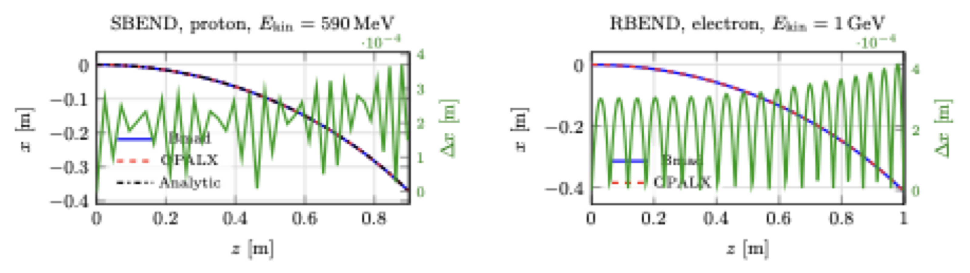
The current implementation has been benchmarked against Bmad for the two simplest no-fringe constant-field cases:

• a proton SBEND with kinetic energy 590 MeV, body length 1 m, and bend angle 45^\circ,
• an electron RBEND with kinetic energy 1 GeV, rectangular body length 1 m, and bend angle 45^\circ.

For the SBEND benchmark, the OPALX trajectory has also been compared with the analytic circular-orbit solution. The comparison plot below shows the current code-to-code agreement. The SBEND benchmark agrees with the analytic endpoint at the exported-design-path level to within approximately (2^{-5},) for DT = 10^{-10} and improves below (10^{-6},) for smaller time steps. The RBEND benchmark now agrees with Bmad to within the displayed plotting resolution for the simple constant-field case.

Figure 3.1: Comparison of the current OPALX SBEND and RBEND benchmarks against Bmad. The SBEND panel also includes the analytic circular-orbit solution. The right axis in each panel shows (x = x_{} - x_{}).

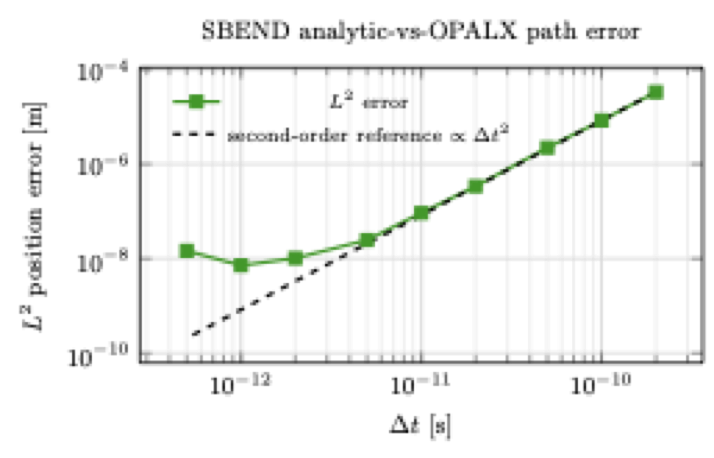
The timestep study for the simple SBEND case is shown below. The reported metric is the discrete path-wise (L^2) error between the OPALX design path and the analytic reference curve, computed over the full bend interval. The dashed reference line shows the expected second-order decay (t^2). The measured convergence is second order over the practical range until it reaches the numerical floor of the current benchmark setup.

Figure 3.2: SBEND timestep study using the path-wise (L^2) error between OPALX and the analytic circular-orbit solution. The dashed line shows the theoretical second-order reference decay.

3.1.7 SBEND and RBEND class structure

The current implementation splits bend handling into a parser-facing OPAL layer and a runtime representation layer. OpalSBend and OpalRBend inherit the common bend attributes and update logic from OpalBend, then instantiate and configure SBendRep and RBendRep respectively.

classDiagram
  direction TB

  class OpalElement

  class OpalBend {
    +clone(name)
    +print(os)
    +deriveAnalyticDipoleCoefficient(Leff, angle)
    +validateAnalyticBendDefinition(name, hasAngle, hasK0, Leff, angle, k0)
  }

  class OpalSBend {
    +OpalSBend()
    +clone(name)
    +update()
  }

  class OpalRBend {
    +OpalRBend()
    +clone(name)
    +update()
  }

  class SBend {
    <<runtime bend>>
  }

  class RBend {
    <<runtime bend>>
  }

  class SBendRep {
    +clone()
    +getGeometry()
    +getField()
    +setField(field)
  }

  class RBendRep {
    +clone()
    +getGeometry()
    +getField()
    +setField(field)
  }

  class PlanarArcGeometry
  class RBendGeometry
  class BMultipoleField

  OpalElement <|-- OpalBend
  OpalBend <|-- OpalSBend
  OpalBend <|-- OpalRBend

  SBend <|-- SBendRep
  RBend <|-- RBendRep

  OpalSBend ..> SBendRep : creates/configures
  OpalRBend ..> RBendRep : creates/configures

  SBendRep *-- PlanarArcGeometry : geometry_m
  SBendRep *-- BMultipoleField : field_m
  RBendRep *-- RBendGeometry : geometry_m
  RBendRep *-- BMultipoleField : field_m

Figure 3.3: Parser-side and runtime-side class structure for the current OPALX-native SBEND and RBEND implementation.

The key distinction is that OpalSBend and OpalRBend are the input and update front ends, while SBendRep and RBendRep own the actual geometry and local normalized multipole field used during tracking.

3.1.8 Example: C-Type Chicane

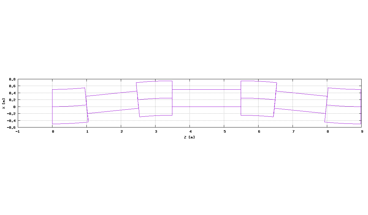
A useful multi-element benchmark for explicit bend placement is a symmetric C-type four-dipole chicane. The example below is deliberately kept at the analytic hard-edge SBEND level: no field maps are used, the four bend bodies are posed explicitly with X, Y, Z, THETA, PHI, and PSI, and the output is checked through the exported element positions and a small off-momentum \(R_{56}\) probe.

The complete runnable input and local post-processing scripts are stored with this chapter:

• test-chicane-1.in
• test-chicane-1_distribution.txt
• check-r56.py

The benchmark uses four equal hard-edge sector bends with physical survey bend signs \[ (+\theta,\,-\theta,\,-\theta,\,+\theta), \] magnetic arc length \(L_b\), outer drift \(D\) between bends 1–2 and 3–4, and central drift \(C\)S between bends 2–3. This is the standard small-angle four-dipole bunch-compressor model used in text book treatments of C-type chicanes (Nguyen et al. 2014; Di Mitri 2018). The numerical constants used here are \[ L_b = 1.0\ \mathrm{m},\qquad \theta = 0.1\ \mathrm{rad},\qquad D = 1.5\ \mathrm{m},\qquad C = 2.0\ \mathrm{m}. \]

For placement, the reference entrance is centered at \((X,Y,Z)=(0,0,0)\), with tangent along global \(+Z\). In the linear approximation we get \[ \rho = \frac{L_b}{\theta}, \] and the other defining constants are \[ \begin{aligned} \Delta x_b &= \rho(1-\cos\theta), &\Delta z_b &= \rho\sin\theta,\\ \Delta x_{b/2} &= \rho\left(1-\cos\frac{\theta}{2}\right), &\Delta z_{b/2} &= \rho\sin\frac{\theta}{2},\\ \Delta x_{r/2} &= \rho\left(\cos\frac{\theta}{2}-\cos\theta\right), &\Delta z_{r/2} &= \rho\left(\sin\theta-\sin\frac{\theta}{2}\right),\\ \Delta x_D &= D\sin\theta, &\Delta z_D &= D\cos\theta . \end{aligned} \] The corresponding names in the imputfile are SB_DX, SB_DZ, SBH_DX, SBH_DZ, RBH_DX, RBH_DZ, DR_DX, and DR_DZ. It then assembles the actual element body origins and monitor locations as B1_X, B1_Z, …, MEXIT_X, MEXIT_Z. This is important because OPALX places an analytic bend by its body origin, not by an entrance edge (BODY pose).

OPALX’s current SBEND angle sign is opposite to the positive-\(X\) survey convention used in this example. Therefore the first and fourth bends use ANGLE = -TH, while the second and third use ANGLE = TH. The element placement remains survey-positive in the named X and Z variables.

The resulting design survey is:

point	(Z) [m]	(X) [m]
B1 entry	0.000000000	0.000000000
B1 exit / D12 begin	0.998334166	0.049958347
B2 entry	2.490840414	0.199708472
B2 exit / D23 begin	3.489174581	0.249666819
B3 entry	5.489174581	0.249666819
B3 exit / D34 begin	6.487508747	0.199708472
B4 entry	7.980014995	0.049958347
B4 exit / MEXIT	8.978349162	0.000000000

Figure 3.4: Projected OPALX element-position export for the analytic four-SBEND C-type chicane. The projection was made from the OPALX-generated test-chicane-1_ElementPositions.py script using the (X)-(Z) plane.

This test does a momentum scan with 5 particles. The launched particles have \[ \delta = \frac{p_z-p_0}{p_0} \in \{-2\times10^{-3},\,-10^{-3},\,0,\,+10^{-3},\,+2\times10^{-3}\}, \] with \(p_0=1957.9509\) in OPALX normalized (\(\beta\gamma\)) units. The small-angle formula for the chicane is \[ R_{56} \simeq -\theta^2\left(\frac{4}{3}L_b + 2D\right) = -4.3334\times10^{-2}\ \mathrm{m}. \] For this monitor convention the local OPALX coordinate has the opposite sign to the usual transport \(R_{56}\) convention, \[ R_{56} = -\frac{d z_{\mathrm{OPALX},\,\mathrm{exit}}}{d\delta}. \] With DT = 1.0e-11 s, the current run gives \[ R_{56} = -4.3114\times10^{-2}\ \mathrm{m}, \] about \[ 2.19 \times 10^{-4}\ \mathrm{m} \] difference from the analytic model.

Run the example from its local directory with:

cd sections/elements/examples/test-chicane-1
/path/to/opalx test-chicane-1.in --info 2
python3 dasta/test-chicane-1_ElementPositions.py --project-to-plane --normal 0 1 0
python3 check-r56.py

3.2 Multipole family

The OPALX MULTIPOLE implementation is the common straight-magnet path for normal and skew magnetic multipole expansions. The present QUADRUPOLE front-end is a convenience wrapper on top of that common path. A dedicated SEXTUPOLE parser-side wrapper is not present in this checkout; sextupole content is therefore expressed through the generic MULTIPOLE coefficient arrays.

3.2.1 Field expansion and conventions

The underlying magnetic field class BMultipoleField (src/Fields/BMultipoleField.h) uses the complex transverse expansion \[ B_y + i B_x = \sum_{m=0}^{N-1} (B_m + i A_m) (x + i y)^m, \] where:

• (m = 0) is the dipole term,
• (m = 1) is the quadrupole term,
• (m = 2) is the sextupole term,
• (B_m) are normal coefficients,
• (A_m) are skew coefficients.

In the abstract multipole interface Multipole (src/AbsBeamline/Multipole.h), the same indexing is used explicitly: n = 0 corresponds to dipole, n = 1 to quadrupole, n = 2 to sextupole, and so on.

For the first three nontrivial components, the transverse magnetic field is:

\[ \text{normal quadrupole:}\qquad B_x = B_1\,y,\qquad B_y = B_1\,x, \]

\[ \text{skew quadrupole:}\qquad B_x = -A_1\,x,\qquad B_y = A_1\,y, \]

\[ \text{normal sextupole:}\qquad B_x = 2 B_2\,x y,\qquad B_y = B_2 (x^2 - y^2), \]

\[ \text{skew sextupole:}\qquad B_x = -A_2 (x^2 - y^2),\qquad B_y = 2 A_2\,x y. \]

These formulas match the host-side field evaluation in src/AbsBeamline/Multipole.cpp.

3.2.2 MULTIPOLE

The parser-side element OpalMultipole (src/Elements/OpalMultipole.cpp) accepts the coefficient arrays:

• KN: normal normalized strengths
• DKN: normal strength errors
• KS: skew normalized strengths
• DKS: skew strength errors

The element semantics are:

• if L != 0, the strengths are interpreted per unit length
• if L == 0, they are interpreted as integrated strengths

At update time, OpalMultipole creates or updates a MultipoleRep (src/BeamlineCore/MultipoleRep.h), copies the element length into its straight geometry, and fills a BMultipoleField plus the runtime coefficient storage in the shared Multipole (src/AbsBeamline/Multipole.h) base.

Internally the generic mapping is:

\[ \texttt{KN}[0] \to \text{dipole},\qquad \texttt{KN}[1] \to \text{quadrupole},\qquad \texttt{KN}[2] \to \text{sextupole}, \]

and likewise for KS.

3.2.3 QUADRUPOLE

The parser-side OpalQuadrupole (src/Elements/OpalQuadrupole.cpp) is not a separate runtime field model. It is a convenience wrapper that instantiates the same MultipoleRep (src/BeamlineCore/MultipoleRep.h) used by MULTIPOLE, but exposes scalar quadrupole attributes instead of full coefficient arrays:

• K1, DK1: normal quadrupole strength and error
• K1S, DK1S: skew quadrupole strength and error

The implementation writes those values into the multipole representation as:

\[ \texttt{KN} = \{0, K_1\},\qquad \texttt{KS} = \{0, K_{1s}\}. \]

So QUADRUPOLE is best understood as a named restricted view of the generic multipole interface with only the (m = 1) term exposed.

3.2.4 SEXTUPOLE

There is currently no dedicated OpalSextupole front-end class in this checkout. The sextupole physics is nevertheless available through the generic MULTIPOLE representation by populating the order-2 coefficients:

\[ \texttt{KN} = \{0, 0, K_2\},\qquad \texttt{KS} = \{0, 0, K_{2s}\}. \]

That means the sextupole is currently a configuration of MULTIPOLE, not a distinct parser-side wrapper parallel to QUADRUPOLE.

For a nonzero body length (L), (K_2) and (K_{2s}) are interpreted as distributed sextupole strengths; for (L = 0), they are integrated strengths, consistent with the generic MULTIPOLE element description.

3.2.5 Runtime geometry and current implementation status

The runtime representation MultipoleRep (src/BeamlineCore/MultipoleRep.h) inherits from Multipole (src/AbsBeamline/Multipole.h) and owns:

• a StraightGeometry
• a BMultipoleField

So the current multipole family described here is a straight-element model with field support over \[ z \in [0, L]. \]

One important current detail from src/AbsBeamline/Multipole.cpp is that the device-side computeField() kernel still contains explicit special cases only for dipole and quadrupole, while the host-side computeFieldHost() implements sextupole and higher orders as well. For the manual this means:

• the interface is generic up to higher order,
• the host/orbit-threader path includes sextupole formulas,
• the current device kernel is still more limited than the abstract interface.

That distinction matters when documenting present implementation status versus intended generality.

3.2.6 Class structure

The current parser-side and runtime-side structure is shown below.

classDiagram
  direction TB

  class OpalElement
  class OpalMultipole {
    +clone(name)
    +print(os)
    +update()
  }
  class OpalQuadrupole {
    +clone(name)
    +print(os)
    +update()
  }

  class Component
  class Multipole {
    +getNormalComponent(n)
    +setNormalComponent(n, v)
    +getSkewComponent(n)
    +setSkewComponent(n, v)
    +apply(...)
    +getField()
    +getGeometry()
  }

  class MultipoleRep {
    +clone()
    +getChannel(key)
    +getField()
    +getGeometry()
    +setField(field)
  }

  class StraightGeometry
  class BMultipoleField

  OpalElement <|-- OpalMultipole
  OpalElement <|-- OpalQuadrupole

  Component <|-- Multipole
  Multipole <|-- MultipoleRep

  OpalMultipole ..> MultipoleRep : creates/configures
  OpalQuadrupole ..> MultipoleRep : creates/configures

  MultipoleRep *-- StraightGeometry : geometry
  MultipoleRep *-- BMultipoleField : field

Figure 3.5: Parser-side and runtime-side class structure for the current MULTIPOLE and QUADRUPOLE implementation. Sextupole content currently enters through the generic MULTIPOLE coefficient path.

In other words, QUADRUPOLE is presently a thin parser-side specialization of the generic multipole path, and sextupole behavior is likewise represented through MultipoleRep, but without a dedicated OpalSextupole wrapper yet.

Di Mitri, S. 2018. “Bunch-Length Compressors.” In Proceedings of the CAS-CERN Accelerator School on Free Electron Lasers and Energy Recovery Linacs, vol. 1. CERN Yellow Reports: School Proceedings. https://doi.org/10.23730/CYRSP-2018-001.361.

Nguyen, D., J. Lewellen, and L. Duffy. 2014. RF Linac for High-Gain FEL: Bunch Compression. US Particle Accelerator School. https://uspas.fnal.gov/materials/14UNM/E_Bunch_Compression.pdf.