Appendix D — Auto-phasing Algorithm
D.1 Standing Wave Cavity
For external RF fields in OPAL-T, the instantaneous field is the interpolated spatial field multiplied by cos(omega t + phi). The energy gain of a particle is therefore
\[ \Delta E(\varphi, r) = q V_0 \int_{z_{\mathrm{begin}}}^{z_{\mathrm{end}}} \cos(\omega t(z,\varphi) + \varphi)\, E_z(z,r)\, dz. \tag{D.1}\]
To maximize the gain, one differentiates with respect to the lag \varphi and sets the derivative to zero. This yields the lag rule
\[ \tan(\varphi) = - \Gamma_1 / \Gamma_2. \tag{D.2}\]
The original appendix defines
\[ \Gamma_1 = \sum_{i=1}^{N-1} \left(1 + \omega \frac{\partial t}{\partial\varphi}\right) \int_{z_{i-1}}^{z_i} \sin\!\left(\omega \left(t_{i-1} + \Delta t_i\frac{z-z_{i-1}}{\Delta z_i}\right)\right) \left(E_{z,i-1} + \Delta E_{z,i}\frac{z-z_{i-1}}{\Delta z_i}\right) dz, \tag{D.3}\]
and
\[ \Gamma_2 = \sum_{i=1}^{N-1} \left(1 + \omega \frac{\partial t}{\partial\varphi}\right) \int_{z_{i-1}}^{z_i} \cos\!\left(\omega \left(t_{i-1} + \Delta t_i\frac{z-z_{i-1}}{\Delta z_i}\right)\right) \left(E_{z,i-1} + \Delta E_{z,i}\frac{z-z_{i-1}}{\Delta z_i}\right) dz. \tag{D.4}\]
Assuming piecewise-linear field and time-of-flight models between samples, the integrals can be evaluated analytically in terms of four coefficients:
\[ \Gamma_{11,i} = -\frac{\cos(\omega t_i) - \cos(\omega t_{i-1})}{\omega\Delta t_i}, \qquad \Gamma_{12,i} = \frac{-\omega\Delta t_i\cos(\omega t_i) + \sin(\omega t_i) - \sin(\omega t_{i-1})}{\omega^2 (\Delta t_i)^2}, \tag{D.5}\]
\[ \Gamma_{21,i} = \frac{\sin(\omega t_i) - \sin(\omega t_{i-1})}{\omega\Delta t_i}, \qquad \Gamma_{22,i} = \frac{\omega\Delta t_i\sin(\omega t_i) + \cos(\omega t_i) - \cos(\omega t_{i-1})}{\omega^2 (\Delta t_i)^2}. \tag{D.6}\]
With these, the appendix rewrites the accumulated sums in a form suitable for an iterative implementation.
D.1.1 Implemented Iterative Idea
The legacy algorithm starts from a guessed kinetic-energy evolution,
K[i] = K[i-1] + (z[i] - z[0]) * q * V;
b[i] = sqrt(1. - 1. / ((K[i] - K[i-1]) / (2.*m*c^2) + 1)^2);
t[i] = t[0] + (z[i] - z[0]) / (c * b[i])
which assumes a roughly linear energy increase proportional to the maximum voltage. From that provisional t(z) model, OPAL computes the lag from Equation D.2, then updates the kinetic energy using the analytic segment formulas,
\[ K_i = K_{i-1} + q\,\Delta z_i \Bigl[ \cos\varphi\,\bigl(E_{z,i-1}(\Gamma_{21,i}-\Gamma_{22,i}) + E_{z,i}\Gamma_{22,i}\bigr) - \sin\varphi\,\bigl(E_{z,i-1}(\Gamma_{11,i}-\Gamma_{12,i}) + E_{z,i}\Gamma_{12,i}\bigr) \Bigr], \tag{D.7}\]
rebuilds the time-of-flight model, and iterates until \varphi converges.
D.2 Traveling Wave Structure
Traveling-wave auto-phasing is slightly more complicated because the field is composed of:
- an entry fringe field
- two standing-wave core contributions with phase offsets
- an exit fringe field
The appendix uses the field map FINLB02-RAC.T7 as the representative traveling-wave example.
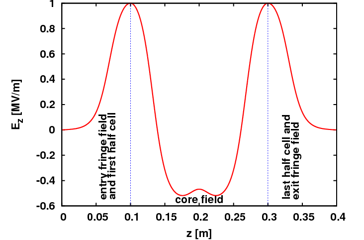
1DDynamic field map used in the traveling-wave auto-phasing discussion.
The corresponding energy gain is written as the sum of four integrals over the entry fringe, two core components, and exit fringe. In the notation of the appendix, the two core contributions are shifted by one cell length s and by phase offsets \varphi_{c1} and \varphi_{c2}.
D.2.1 Example
The legacy example is:
FINLB02_RAC: TravelingWave, L=2.80, VOLT=14.750*30/31,
             NUMCELLS=40, FMAPFN="FINLB02-RAC.T7",
             ELEMEDGE=2.67066, MODE=1/3,
             FREQ=1498.956, LAG=FINLB02_RAC_lag;
From this, the appendix derives
\[ V_{\mathrm{core}} = \frac{V_0}{\sin(2\pi/3)} = \frac{2V_0}{\sqrt{3}}, \qquad \varphi_{c1} = \frac{\pi}{6}, \qquad \varphi_{c2} = \frac{\pi}{2}, \tag{D.8}\]
and an exit-fringe phase offset determined by NUMCELLS and MODE.
D.2.2 Alternative Approach for Traveling-Wave Structures
In the ultra-relativistic limit, where beta changes only weakly along the structure, the time-of-flight can be approximated linearly,
\[ t(z,\varphi) \approx \frac{z}{\beta c} + t_0. \tag{D.9}\]
For the traveling-wave example, the appendix then rewrites the derivative condition in terms of periodic core and fringe fields over a period 3 s, and shows how the expression simplifies because \omega/(\beta c) \approx 10\pi. The final reduced condition is expressed as a convolution,
\[ 0 \equiv \int_0^{3s} g(\xi-z)\,\bigl(G(z) - 26 H(z)\bigr)\,dz = \mathcal{F}^{-1}\!\left(\mathcal{F}(g)\,\bigl(\mathcal{F}(G)-26\mathcal{F}(H)\bigr)\right), \tag{D.10}\]
with the phase relation
\[ -\frac{\omega}{\beta c}\,\xi = \varphi. \tag{D.11}\]
The appendix also uses the trigonometric identity
\[ \sin(a+\pi+\pi/6) + \sin(a+\pi-\pi/6) = -\sqrt{3}\,\sin(a), \tag{D.12}\]
which is the final algebraic step that collapses the two core terms into the reduced convolution form.